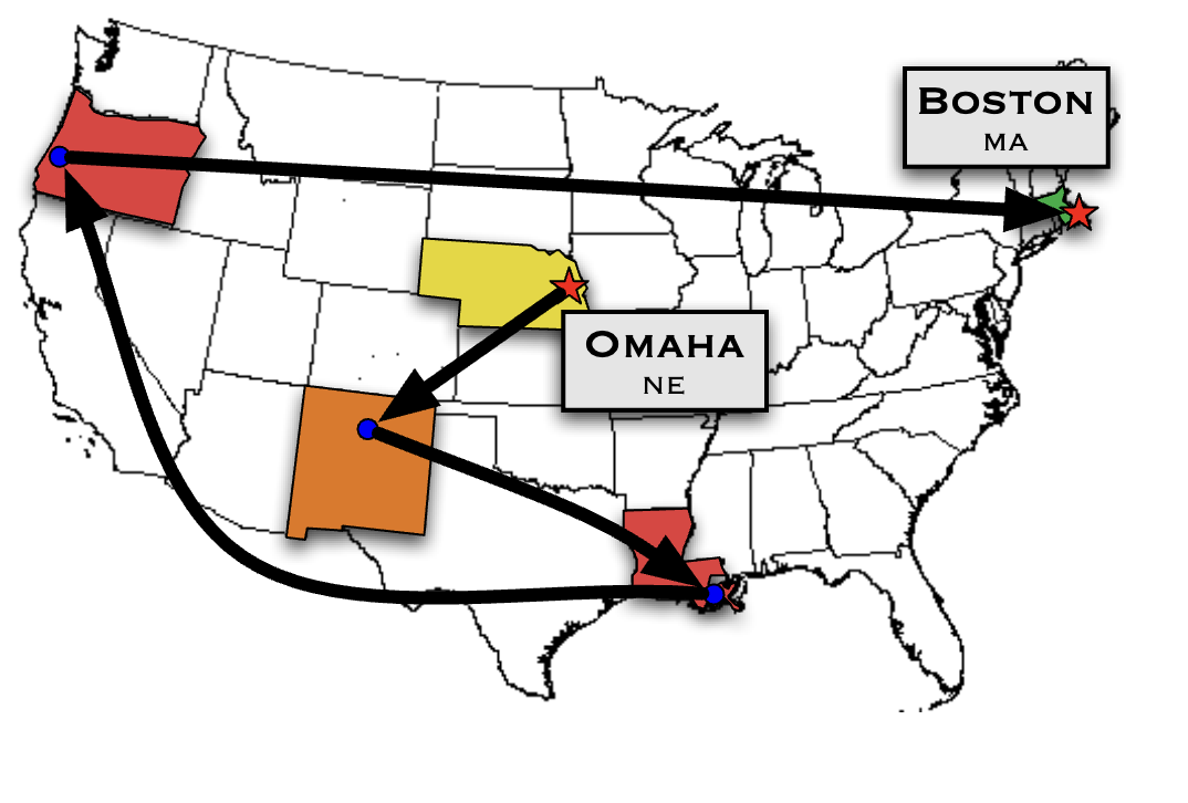
Why are people in the world connected by a small number of steps?
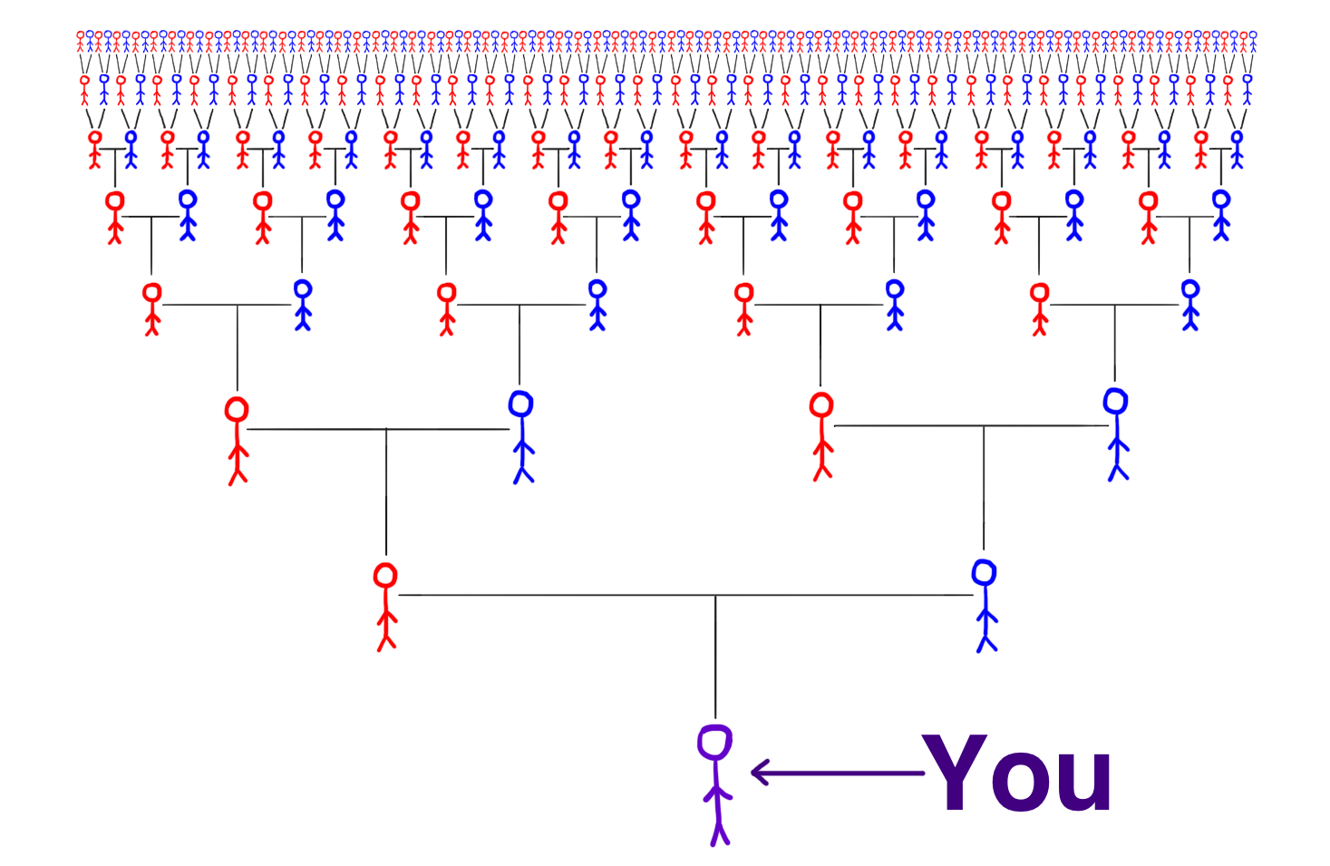
Think about your family tree:
How many ancestors do you have in each generation?
1 generation back (parents)
5 generations back?
10 generations back?
Ancestors double each generation \(\rightarrow\)exponential growth.
In social networks, having more than 2 friends means you can reach billions in just a few steps. \(\leftarrow\)does this explain the small-world property 🤔?
Wait, think about 100 generations back
100 generation \(\simeq\) 2000 years
The number of ancestors is \(2^{100} \simeq 10^{30}\)
But, population in 2000 years ago was only 200 million.
Then, what’s wrong with the estimate 🤔?
The family tree isn’t a true tree—many ancestors overlap (due to incest).
Local connections are more common in social networks—your friends are also friends with each other.
Exponential growth alone doesn’t explain short social distances!
Key question
If people are connected locally, then our social networks are NOT small-world.
But observations show that it is small-world.
So, how can a network have lots of local connections and still remain globally compact 🤔?
Let’s make it clear what we mean by local and global connections.
Clustering Coefficient (1)
Local clustering asks: given all your friends, how many of triangles you and your friends form, relative to the maximum possible number of triangles?
\[
C_i = \dfrac{\text{\# of triangles involving } i \text{ and its neighbors}}{\text{\# of edges possibly exist in the neighborhood of } i}
\]
Node A has 5 neighbors
Triangles with A: 2
Possible triangles: \(\binom{5}{2} = 10\)
\(C_A = 2/10 = 0.2\)
What are the local clustering coefficients of A, B and C?
\[
C_i = \dfrac{\text{# of triangles involving } i \text{ and its neighbors}}{\text{# of edges possibly exist in the neighborhood of } i}
\]
A: \(2/6 = 1/3\)
B: \(1/3 = 1/3\)
C: \(0\)
Clustering Coefficient (2)
Average clustering coefficient is the average of the local clustering coefficients of all nodes.
Global clustering coefficient focuses on the total number of triangles in the network.
\[
C = \frac{3 \times \text{number of triangles}}{\text{number of connected triplets}} = \frac{3 \times \text{number of triangles}}{\sum_{i} k_i(k_i-1)/2}
\]
where \(k_i\) is the degree of node \(i\).
Connected triplets = Three nodes joined by at least two edges. When counting, we distinguish the triplets by the node that is centered. A triangle counts as three triplets. A node with degree \(k\) has \(k(k-1)/2\) triplets.
Closed triplet (left) and open triplet (right)
Three types of clustering coefficients:
Local clustering coefficient\(\rightarrow\) Density of triangles in a node’s neighborhood
Average clustering coefficient\(\rightarrow\) Average of the local clustering
Global clustering coefficient\(\rightarrow\) Density of triangles in the entire network
Question:
If a network has a high global clustering coefficient, does it necessarily have a high average local clustering coefficient?
If not, can you draw a network with high global clustering but low average local clustering coefficient?
Average Path Length (1)
Now, let’s quantify the global connectivity via the average path length.
Distance between two nodes \(i\) and \(j\) is the minimum number of edges you need to traverse to get from one node to the other
Let’s find the distance between A and D:
Path 1: A \(\rightarrow\) B \(\rightarrow\) D (2 edges)
Path 2: A \(\rightarrow\) C \(\rightarrow\) D (2 edges)
Path 3: A \(\rightarrow\) C \(\rightarrow\) B \(\rightarrow\) D (3 edges)
Even though there are multiple paths, the distance from A to D is 2 edges.
Average Path Length (2)
Average path length \(L\) is the average distance between any two nodes:
import igraphedge_list = [(0, 1), (1, 2), (0, 2), (0, 3)]g = igraph.Graph() # Create an empty graphg.add_vertices(4) # Add 4 verticesg.add_edges(edge_list) # Add edges to the graph
Plot the graph.
import matplotlib.pyplot as pltfig, ax = plt.subplots(figsize=(5, 5))# Draw the graph on the matplotlib axes using igraphigraph.plot( g, bbox=(50, 50), vertex_label=list(range(4)), target=ax,)
Path
Simple paths:
g.get_all_simple_paths(2, to=3)
Shortest path:
# Shortest pathg.get_shortest_paths(2, to=3)
Distance:
# Distanceg.distances(2, 3)
Connected Components
Find connected components:
components = g.connected_components()
Membership:
components.membership
Size:
components.size
The largest connected component:
components.giant()
Clustering coefficient
Local clustering coefficient:
g_cluster.transitivity_local_undirected()
Average clustering coefficient:
g_cluster.transitivity_avglocal_undirected()
Global clustering coefficient:
g_cluster.transitivity_undirected()
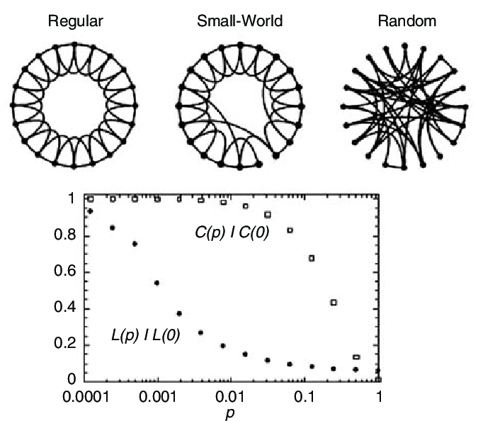
Watts-Strogatz Model
n_ws =30# Number of nodesk_ws =6# Number of nearest neighbors in the ring latticep_rewire =0.1# Probability of rewiring each edgeg_smallworld = igraph.Graph.Watts_Strogatz( dim=1, size=n_ws, nei=k_ws //2, p=p_rewire,)
Compute the small-worldness \(\sigma\) using the formula below: