Advanced Topics in Network Science

Lecture 07: Random Walks Sadamori Kojaku

What to Learn 📚

🎲 Random walks as a powerful tool in network analysis
🧮 Characterization of random walks in networks
🌟 Steady state distribution, and dynamic behavior
🔗 Connection to centrality measures and community detection

Have you ever played this game? 🎮

Ladder Lottery Game 🪜

Choose a line.
Move along the line, cross the horizontal lines if you hit them.
Stop at the end of the line.
You’ll win if you hit a treasure at the end of the line.

Suppose you know where is the treasure is located. Think a strategy to maximize your winning probability 🤔.

Interactive demo 👾

Answer

Choose the line above the treasure.

Why?

Suppose that there is no horizontal line. You’ll win if you choose the line above the treasure.
Now, consider adding few horizontal lines. You’ll only move other lines few times, and you’ll end up with being on the line centered around the treasure with high probability.
The chance of winning “diffuses” as the number of horizontal lines increases, with limit close to uniform.

This is a network!

Random Walks in Networks 🌐

🚶‍♀️ Simple process: Start at a node, randomly move to neighbors
🏙️ Analogy: Drunk person walking in a city
Interestingly, this random process captures many important properties of networks
Unifies different concepts in network science, e.g., centrality, community structure

Interactive Demo: Random Walk

Random Walk Simulator

When the random walker makes many steps, where does it tend to visit most frequently?
When the walker makes only a few steps, where does it tend to visit?
Does the behavior of the walker inform us about centrality of the nodes?
Does the behavior of the walker inform us about communities in the network?

Pen and Paper (and a bit of coding) Exercises ✍️

Pen and Paper Exercise (and a bit of coding)

Mathematical Foundations of Random Walks 🧮

Transition Probability Matrix 📊

Transition probability

\[ P_{ij} = \frac{A_{ij}}{k_i} \]

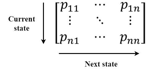
where \(A_{ij}\): Adjacency matrix element, and \(k_i\): Degree of node \(i\).

In matrix form

\[ \mathbf{P} = \mathbf{D}^{-1}\mathbf{A} \]

where \(\mathbf{D}\): Diagonal matrix of node degrees.

Stationary Distribution 📈

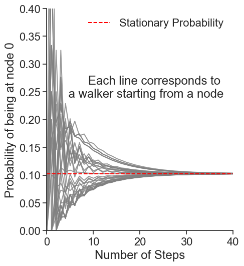
Let us consider a random walk on an undirected network starting from a node. After sufficiently many steps, where will the walker be?
Let \(x_i(t)\) be the probability that a random walker is at node \(i\) at time \(t\).
After many steps, \(\lim_{t\to\infty} x_i(t) = \pi_i\), which is time invariant, \(\pi_i\) is called the stationary distribution
At stationary state,

\[ {\bf \pi} = {\bf \pi P} \]

What is the solution?

Stationary Distribution

This is the eigenvalue problem.

\[ {\bf \pi} = {\bf \pi P} \]

One of the left-eigenvector of \({\bf P}\) is the stationary distribution

Question: - There are \(N\) left-eigenvectors for a network with \(N\) nodes. Which one represents the stationary distribution?

Coding Exercise:

Create a karate-club graph.

import igraph as ig
import numpy as np

g = ig.Graph.Famous("Zachary") # Load the Zachary's karate club network
A = g.get_adjacency_sparse() # Get the adjacency matrix

Task 1: Create a line plot of the probability distribution of the random walker over the nodes as a function of the number of steps. Create the plot for walkers starting from node 0, 32, or 6.

Task 2: Compute the stationary distribution using the eigenvector problem \({\bf \pi} = {\bf \pi P}\). You may want to use np.linalg.eig to compute the (left) eigenvectors and eigenvalues of the matrix \({\bf P}\).

Task 3: Compare the stationary distribution with the degree distribution.

Transient state

Transient State

Transient state captures the local structure around the starting node.

e.g., community structure, cycles, degree assortativity, etc.

When does the transient state end?

👉 Mixing Time

\(t_{\text{mix}} = \min\{t : \max_{{\bf x}(0)} \|{\bf x}(t) - {\bf \pi}\|_{1} \leq \epsilon\}\)

Time to reach the stationary distribution within a certain tolerance \(\epsilon\).

Mixing Time

Random walk distribution \({\bf x}(t)\) at time \(t\) is given by

\[ {\bf x}(t) = {\bf x}(0) \mathbf{P}^t. \]

where

\({\bf x}(0)\): Initial state vector
\({\bf x}(t)\): State vector at time \(t\)

The mixing time depends on the initial state \({\bf x}(0)\) and \({\bf P}^t\).

The network structure is encapsulated in \({\bf P}\). But this does not tell us what structure in \({\bf P}\) affects the mixing time. 🤔

What’s your expectation?

What network structure affects the mixing time, and in what way?

How does this structure show up in the transition probability matrix \({\bf P}\)?

\[ {\bf x}(t) = {\bf x}(0) \mathbf{P}^t. \]

Let’s arm ourselves with some matrix algebra 🧰

Diagonalizability

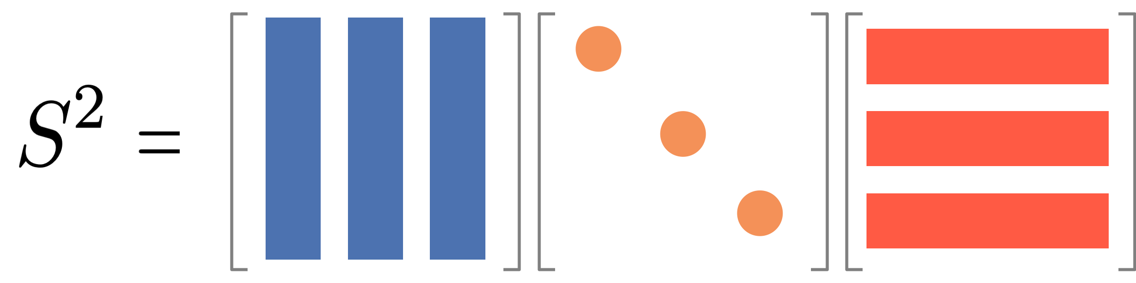
Diagonalizable matrix: A matrix \(\mathbf{S}\) is diagonalizable if \({\bf S}\) can be represented as \(\mathbf{S} = \mathbf{Q}\mathbf{\Lambda}\mathbf{Q}^{-1}\), where \(\mathbf{Q}\) is an invertible matrix and \(\mathbf{\Lambda}\) is a diagonal matrix of eigenvalues.

Exercise: Diagonalizabilty helps us to compute a power of a matrix easily. Compute the power \({\bf S}^2\) of diagonalizable matrix \({\bf S} = \mathbf{Q}\mathbf{\Lambda}\mathbf{Q}^{-1}\).

Power of Diagonalizable Matrix

\({\bf S}^2 = \mathbf{Q}\mathbf{\Lambda}\mathbf{Q}^{-1} \mathbf{Q}\mathbf{\Lambda}\mathbf{Q}^{-1} = \mathbf{Q}\mathbf{\Lambda}^2\mathbf{Q}^{-1}\)
In general, \({\bf S}^t = \mathbf{Q}\mathbf{\Lambda}^t\mathbf{Q}^{-1}\)

Is the transition matrix diagonalizable? Yes 🙂!

Let’s introduce a new matrix \(\mathbf{\bar A}\) called the normalized adjacency matrix.

\[ \mathbf{\bar A} = \mathbf{D}^{-\frac{1}{2}} \mathbf{A} \mathbf{D}^{-\frac{1}{2}} \]

\({\bf D}\) is a diagonal matrix of node degrees, i.e.,

\[ \mathbf{D} = \begin{pmatrix} k_1 & 0 & \cdots & 0 \\ 0 & k_2 & \cdots & 0 \\ \vdots & \vdots & \ddots & \vdots \\ 0 & 0 & \cdots & k_N \end{pmatrix} \]

The transition matrix \(\mathbf{P}\) can be rewritten as \[ \begin{aligned} \mathbf{P} &= \mathbf{D}^{-1} \mathbf{A} \\ & = \mathbf{D}^{-\frac{1}{2}} \left( \mathbf{D}^{-1/2} \mathbf{A} \mathbf{D}^{-1/2} \right) \mathbf{D}^{\frac{1}{2}} \\ &= \mathbf{D}^{-\frac{1}{2}} \mathbf{\bar A} \mathbf{D}^{\frac{1}{2}} \end{aligned} \]

Matrix \(\mathbf{\bar A}\) is symmetric (since the network is undirected) and therefore diagonalizable:

\[ \mathbf{\bar A} = \mathbf{Q} \mathbf{\Lambda} \mathbf{Q}^{\top}, \]

where \(\mathbf{\Lambda}\) is a diagonal matrix of eigenvalues, and \(\mathbf{Q}\) is a matrix of eigenvectors of \(\mathbf{\bar A}\).

Let’s express \(\mathbf{P}^2\) using \(\mathbf{D}\), \(\mathbf{Q}\), and \(\mathbf{\Lambda}\).

\[ \begin{aligned} \mathbf{P}^2 &= \left( \mathbf{D}^{-\frac{1}{2}} {\bf \overline A} \mathbf{D}^{\frac{1}{2}} \right)^2 \\ &= \mathbf{D}^{-\frac{1}{2}} \mathbf{\overline A} \mathbf{D}^{\frac{1}{2}} \mathbf{D}^{-\frac{1}{2}} \mathbf{\overline A} \mathbf{D}^{\frac{1}{2}} \\ & = \mathbf{D}^{-\frac{1}{2}} {\bf \overline A}^2 \mathbf{D}^{\frac{1}{2}} \\ &= \underbrace{\mathbf{D}^{-\frac{1}{2}} \mathbf{Q}}_{{\bf Q}_L} {\bf \Lambda}^2 \underbrace{\mathbf{Q}^\top \mathbf{D}^{\frac{1}{2}}}_{{\bf Q}^\top _R}\\ \end{aligned} \]

where we defined:

\[ {\bf Q}_L = \mathbf{D}^{-\frac{1}{2}} \mathbf{Q}, \quad {\bf Q} _R = \mathbf{D}^{\frac{1}{2}} \mathbf{Q} \]

Question: What would you get by computing the product \({\bf Q}_L ^\top {\bf Q}_R\)?

Transition matrix is diagonalizable

\[ {\bf Q}_L ^\top {\bf Q}_R = \mathbf{I} \]

So the transition matrix \(\mathbf{P}\) is diagonalizable 🙂!

\[ \mathbf{P} = {\bf Q}_L \mathbf{\Lambda} \mathbf{Q}_R \]

where

\[ {\bf Q}_L = \mathbf{D}^{-\frac{1}{2}} \mathbf{Q}, \quad {\bf Q} _R = \mathbf{D}^{\frac{1}{2}} \mathbf{Q} \]

with \(\mathbf{Q}_R \mathbf{Q}_L^{-1} = \mathbf{I}\). This means that

\[ {\bf P}^t = {\bf Q}_L \mathbf{\Lambda}^t \mathbf{Q}_R \]

Mixing Time

Let’s put \({\bf P}^t = {\bf Q}_L \mathbf{\Lambda}^t \mathbf{Q}_R\) into the random walk equation:

\[ \begin{aligned} {\bf x}(t) &= {\bf x}(0) \mathbf{P}^t \\ &= {\bf x}(0) \mathbf{Q}_L \mathbf{\Lambda}^t \mathbf{Q}_R \end{aligned} \]

In element-wise, we have

\[ \begin{pmatrix} x_1(t) \\ x_2(t) \\ \vdots \\ x_N(t) \end{pmatrix} = \sum_{\ell=1}^N \left[ \lambda_\ell^t \langle\mathbf{q}^{(R)}_{\ell}, \mathbf{x}(0) \rangle \begin{pmatrix} q^{(L)}_{\ell 1} \\ q^{(L)}_{\ell 2} \\ \vdots \\ q^{(L)}_{\ell N} \end{pmatrix} \right] \]

Mixing Time

\[ \begin{pmatrix} x_1(t) \\ x_2(t) \\ \vdots \\ x_N(t) \end{pmatrix} = \sum_{\ell=1}^N \left[ \color{red}{\lambda_\ell^t} \langle\mathbf{q}^{(R)}_{\ell}, \mathbf{x}(0) \rangle \begin{pmatrix} q^{(L)}_{\ell 1} \\ q^{(L)}_{\ell 2} \\ \vdots \\ q^{(L)}_{\ell N} \end{pmatrix} \right] \]

\(\lambda_i \leq 1\) (the blue balls) with equality holds for the largest eigenvalue \(\lambda_1 = 1\).
When \(t \rightarrow \infty\), only the largest eigenvalue \(\lambda_1\) survives
Other eigenvalues \(\lambda_i\) decay exponentially as \(t\) increases
The second largest eigenvalue \(\lambda_2\) most significantly affects the mixing time.

Mixing Time and Relaxation Time

The relaxation time \(\tau\) is given by

\[ \tau = \frac{1}{1-\lambda_2} \]

where \(\lambda_2\) is the second largest eigenvalue of the normalized adjacency matrix \(\mathbf{\bar A}\).

Relaxation time \(\tau\) is a convenient reference for the mixing time, as it bounds the mixing time.

\[ t_{\text{mix}} < \tau \log \left( \frac{1}{\epsilon \min_{i} \pi_i} \right) \]

Coding Exercise

Task 1: Construct the adjacency matrices of two graphs as follows:

Task 2: Compute the normalized adjacency matrix \({\bf \overline A} = \mathbf{D}^{-\frac{1}{2}} \mathbf{A} \mathbf{D}^{-\frac{1}{2}}\), where \(\mathbf{D}\) is the degree diagonal matrix.

Task 3: Compute the relaxation time \(\tau = \frac{1}{1-\lambda_2}\) using the second largest eigenvalue \(\lambda_2\) of the normalized adjacency matrix.

Relationship between Random Walks, Modularity, and Centrality 🌟

https://skojaku.github.io/adv-net-sci/m07-random-walks/unifying-centrality-and-communities.html