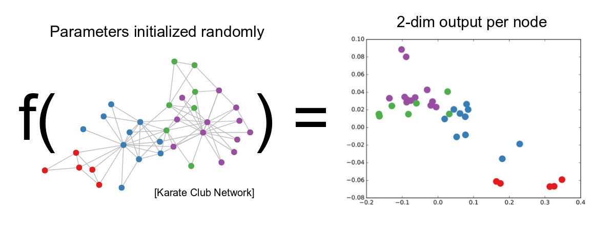
import igraph as ig
import numpy as np
import matplotlib.pyplot as plt
import seaborn as sns

A = ig.Graph.Famous("Zachary").get_adjacency_sparse() # Load the karate club network
eigvals, eigvecs = np.linalg.eig(A.toarray()) # Eigenvalues and eigenvectors
eigvals, eigvecs = np.real(eigvals), np.real(eigvecs)

fig, axes = plt.subplots(1,4, figsize=(15,3))

for i in range(3):
    u = eigvecs[:, i].reshape((-1,1))
    lam = eigvals[i]

    basisMatrix = u @ u.T

    sns.heatmap(basisMatrix, ax=axes[i+1], cmap="coolwarm", center=0)
    axes[i+1].set_title(f"Lambda={lam:.2f}")
sns.heatmap(A.toarray(), ax=axes[0], cmap="coolwarm", center=0)
axes[0].set_title("Adjacency Matrix")
plt.show()Solution for general d dimensional case
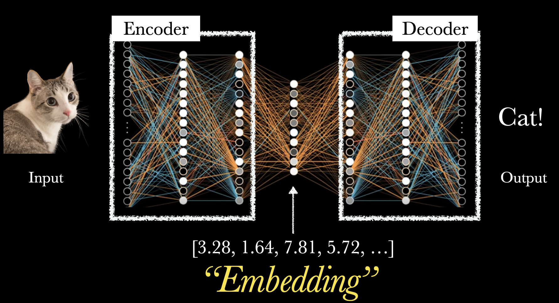
Network Embedding 🌐
- Task: Embed a network into a low-dimensional vector space
- Embedding can recover the network with high accuracy
- Embedding should be low-dimensional
Question:
How would you do that? What approaches would be viable?
Why eigenvectors?
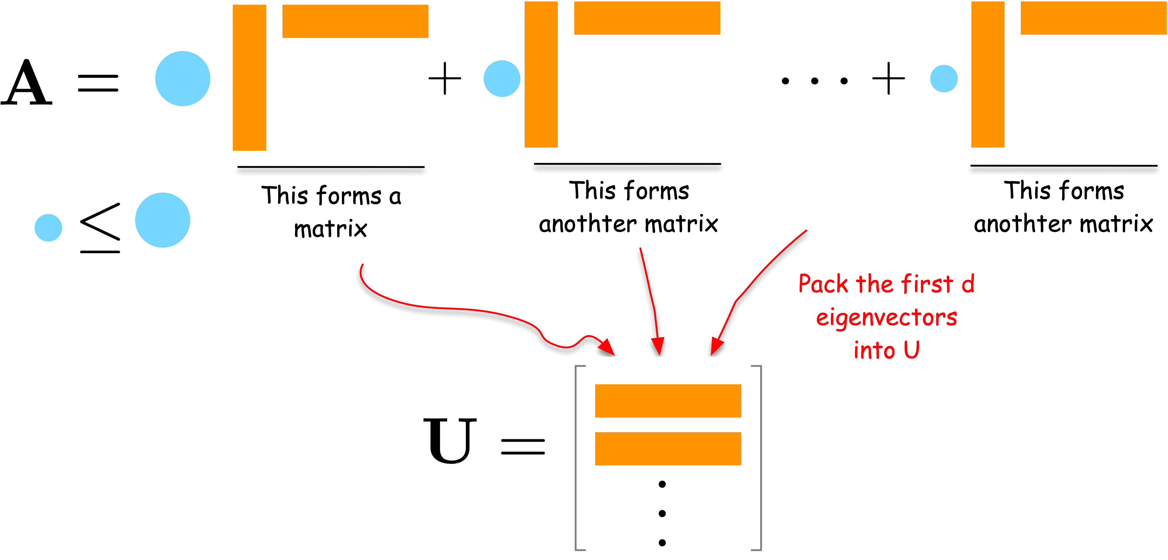
Intuition behind eigenvectors

The d eigenvectors associated with the largest d eigenvalues give the optimal solution that minimizes the reconstruction error for the d dimensional case.
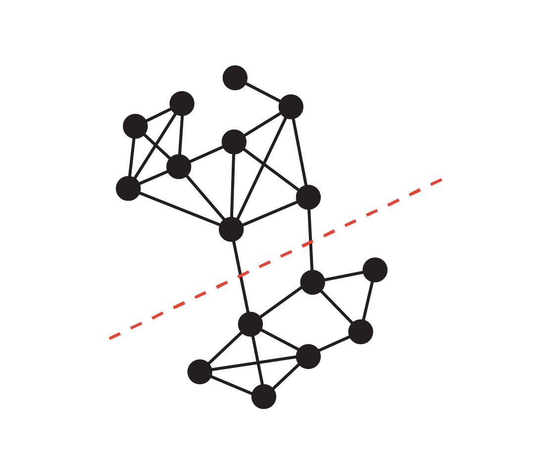
Graph cut Problem
Graph cut Problem ✂️
Disconnect a graph into two components by cutting the minimum number of edges
\min_{Q,S} \text{cut}(Q,S) = \sum_{i \in Q} \sum_{j \in S} A_{ij}
where |Q \cup S| = N, \quad Q \cap S = \emptyset
This has a close relationship with the Laplacian matrices L and L_n given by
L = D - A, \quad L_n = I - D^{-1/2} A D^{-1/2}
where D is the degree matrix and A is the adjacency matrix.
Neural networks for embedding
How can I apply neural networks to embedding?
- Run random walks
- Treat the walks as sentences
- Apply neural networks to predict temporal correlations between words
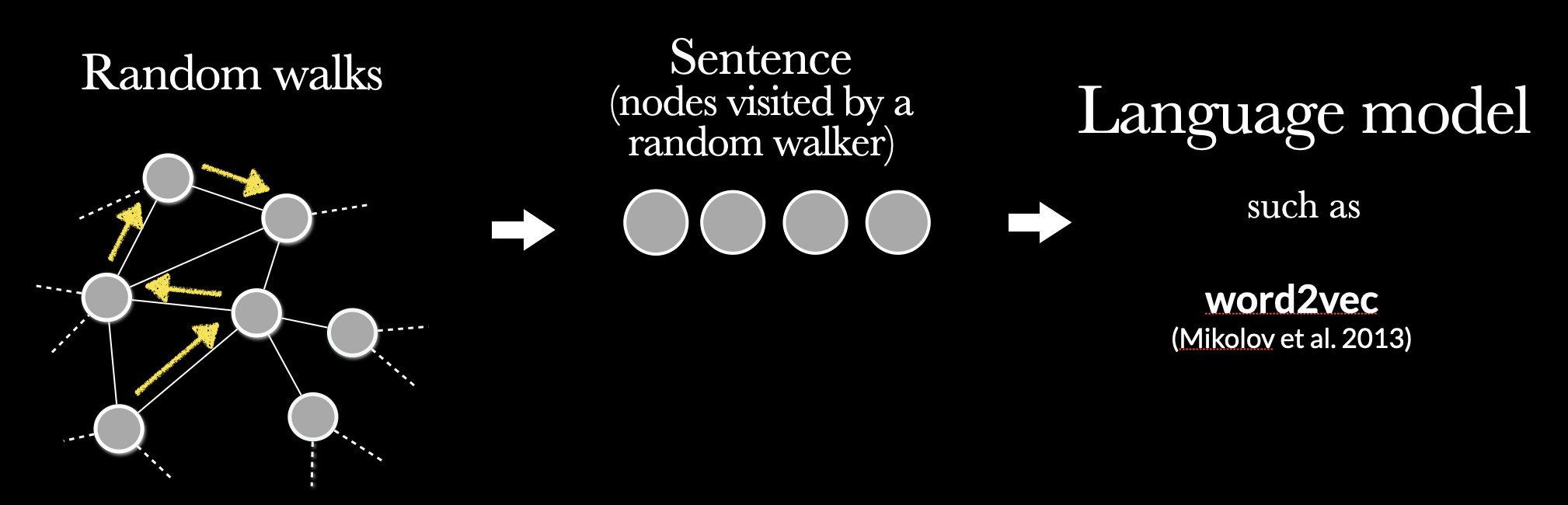
DeepWalk & node2vec: Use word2vec to learn node embeddings from random walks
Note:
This is one way. Another popular way is to use convolution inspired from image processing.
CBOW Model
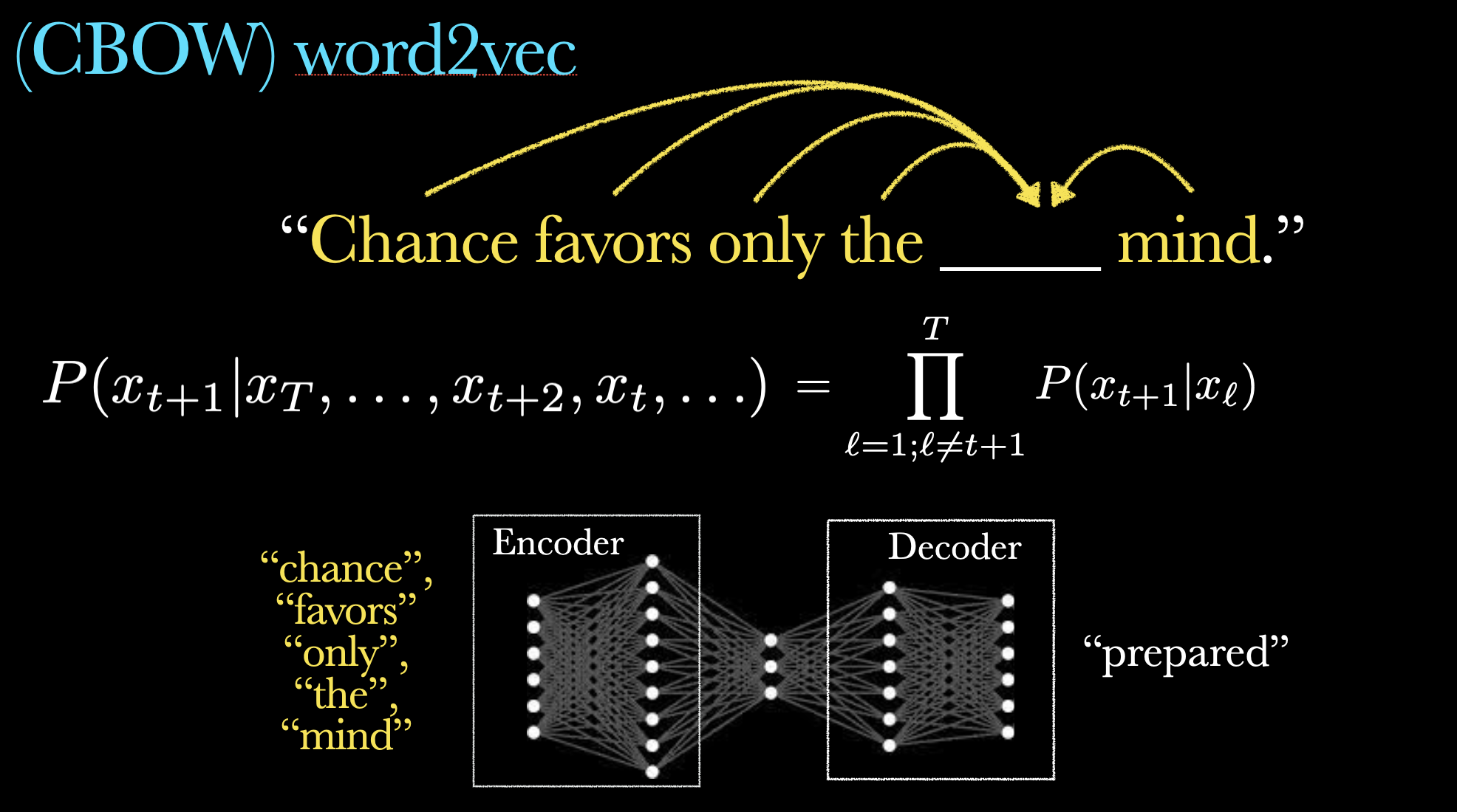
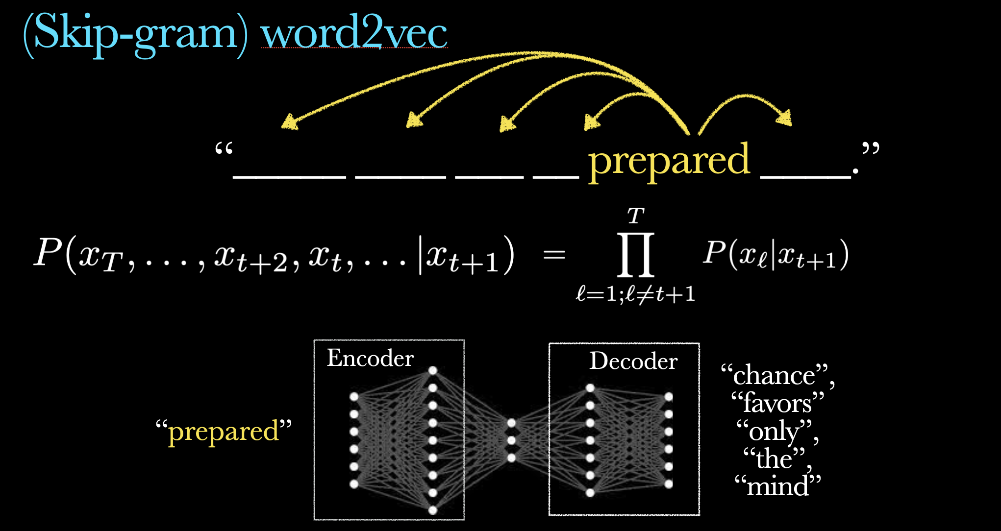
Skipgram
node2vec 📝

- Learn multi-step transition probabilities of random walks
- High probability ~ close in the embedding space
Note:
Precisely speaking, this is not an accurate model description. node2vec is trained on a biased training algorithm. Consequently, two frequently co-visited nodes are not always embedded closely. See paper
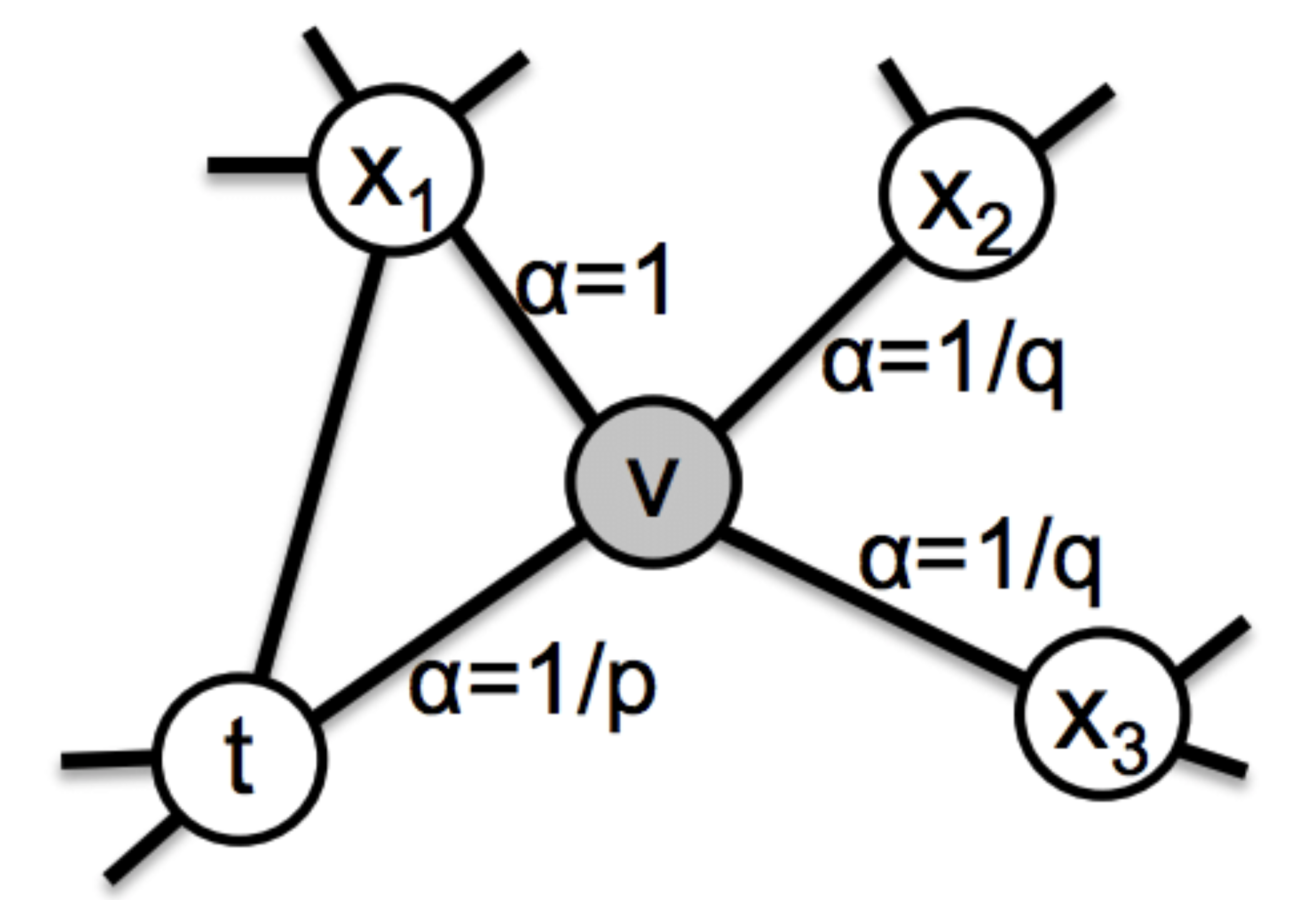
node2vec random walks
Biased Random Walk:
\begin{align*} P(x_{t+1}|x_t, x_{t-1}) \propto\begin{cases} \frac{1}{p} & \text{Return to } x_{t-1} \\ 1 & \text{Move to a neighbor $x_{t+1}$ directly connected to } x_{t-1} \\ \frac{1}{q} & \text{Move to a neighbor $x_{t+1}$ *not* directly connected to } x_{t-1} \end{cases} \end{align*}
Parameters:
- p: Return parameter (lower = more backtracking)
- q: Exploration parameter (lower = more exploration)
which control the walker to move away from the previous node or stay locally.
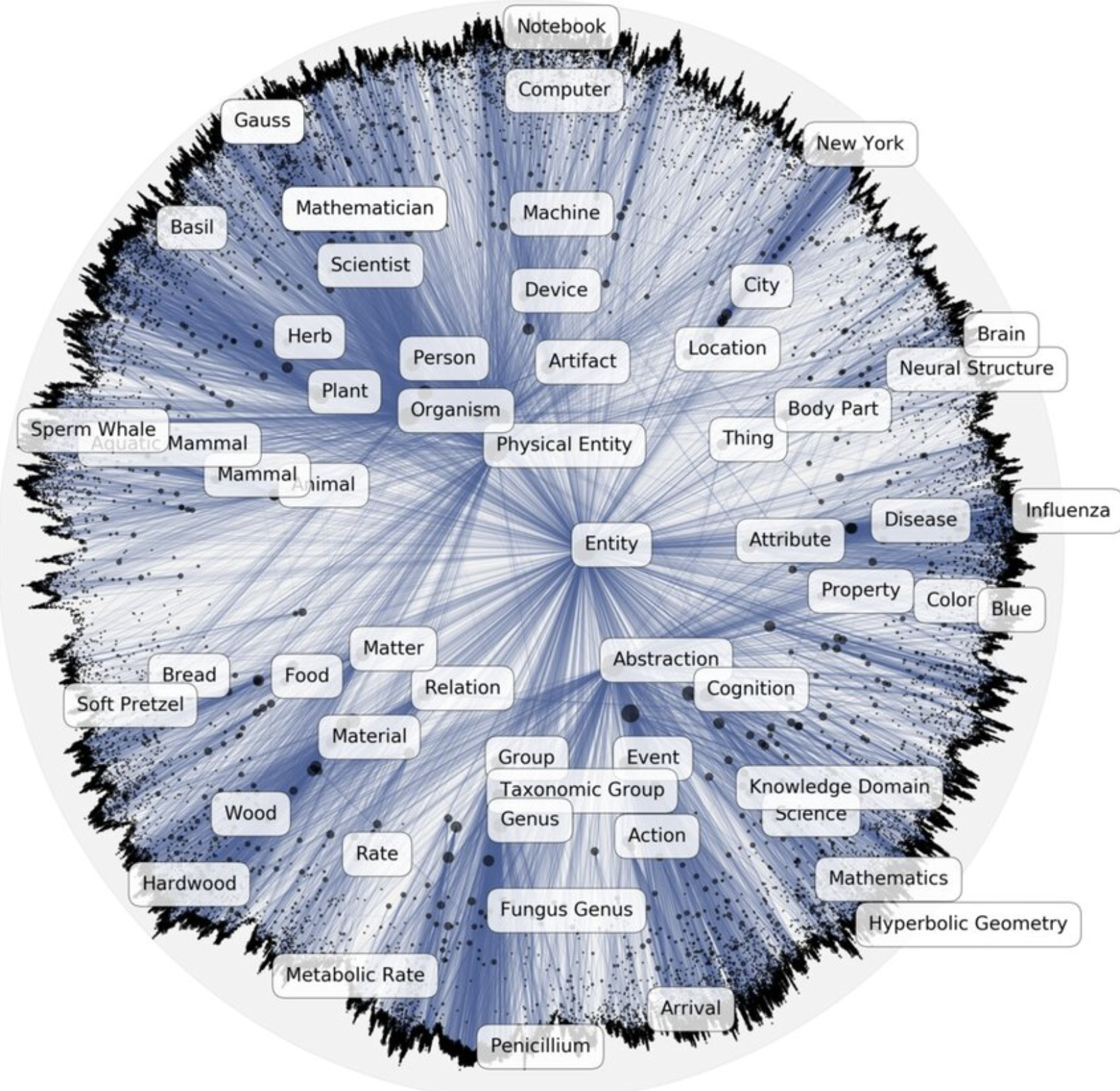
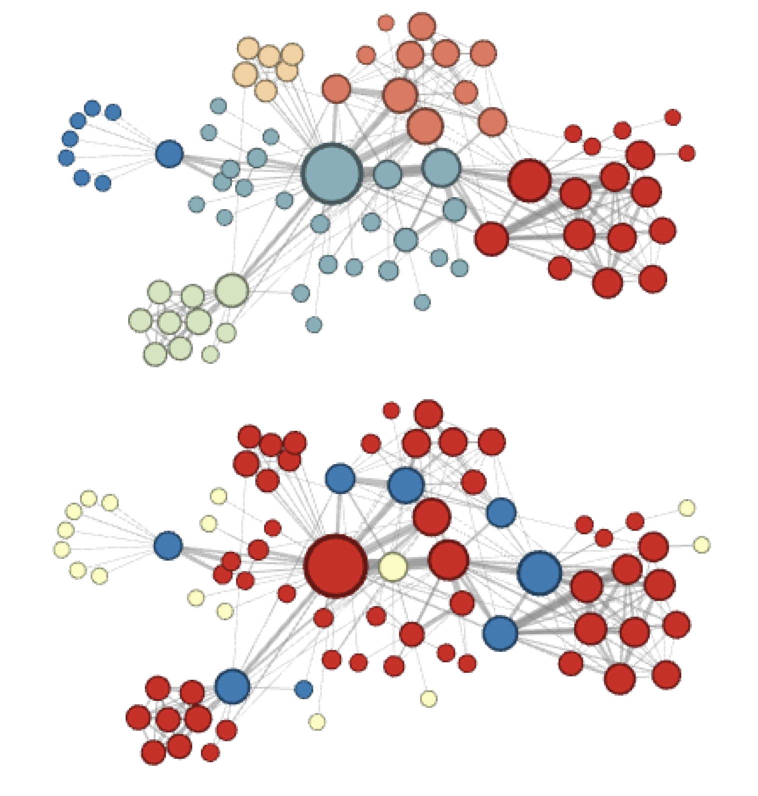
Example: Les Misérables Network 📚
Complementary visualizations of Les Misérables coappearance network generated by node2vec with label colors reflecting homophily (top) and structural equivalence (bottom).
The Challenge with Euclidean Space
- Problem: Real networks have
- Hierarchical structures
- Scale-free properties
- Strong clustering + small-world
- Issue: In flat (Euclidean) space, volume grows polynomially with radius
- But: Tree-like hierarchies grow exponentially
- This is a fundamental mismatch!

What is Hyperbolic Space?
Hyperbolic geometry = curved space with negative curvature
Key Property:
Volume grows exponentially with radius—just like trees!
This naturally captures:
- Scale-free degree distributions
- Strong clustering
- Small-world property
- Self-similarity
Poincaré disk: hyperbolic space visualized in a circle
Answer: It’s Both! ⚖️
Discovery:
Networks grow by balancing two factors:
- Popularity: Connect to well-established nodes
- Similarity: Connect to similar nodes
This optimization naturally emerges in hyperbolic space!
- Popularity → radial position (birth time)
- Similarity → angular distance
- New connections → hyperbolically closest nodes

The Core Model: Popularity × Similarity
Network Generation Process:
- At each time t = 1, 2, 3, \dots, add a new node t
- Each node t gets coordinates:
- Random angular position on a circle, \theta_t
- Radial position based on birth time, r_t = \ln t (older = more popular)
- New node t connects to the m nodes that minimize:
s \cdot \theta_{st} \quad \text{for } s < t
Key property: In this space, the rule “minimize s \cdot \theta_{st}” is mathematically equivalent to connecting to the m hyperbolically closest nodes.
1. Poincaré Ball Model 🔮
Points lie within unit ball: \|\mathbf{x}\| < 1
Distance formula:
d_P(\mathbf{u}, \mathbf{v}) = \text{arcosh}\left(1 + 2\frac{\|\mathbf{u} - \mathbf{v}\|^2}{(1 - \|\mathbf{u}\|^2)(1 - \|\mathbf{v}\|^2)}\right)
Properties:
- Intuitive visualization
- Geodesics = circular arcs
- Requires complex Riemannian optimization
Shapes appear to shrink near boundary, but they’re all the same hyperbolic size!
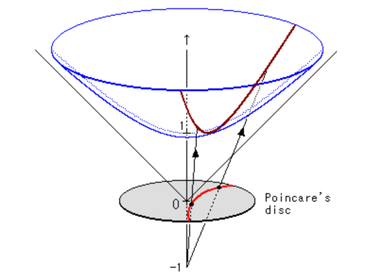
2. Lorentzian (Hyperboloid) Model 🎯
Points lie on hyperboloid in Minkowski space
Lorentzian inner product:
\langle\mathbf{x}, \mathbf{y}\rangle_L = -x_0 y_0 + x_1 y_1 + \cdots + x_n y_n
Distance formula:
d_L(\mathbf{u}, \mathbf{v}) = \text{arcosh}(-\langle\mathbf{u}, \mathbf{v}\rangle_L)
Advantage: More efficient optimization (gradients in Euclidean ambient space)
Hyperboloid projects onto Poincaré disk
What do hyperbolic embeddings look like?