Core Concepts
1 What to learn in this module
In this module, we will learn community detection, one of the most widely-used yet controversial techniques in network analysis. We will learn:
- What is community structure in networks?
- How to operationalize community structure?
- How to find communities in networks?
- Limitations of community detection
- Keywords: community detection, assortativity, modularity, resolution limit, rugged landscape, random graph, label switching algorithm, Louvain algorithm, stochastic block model, the configuration model.
Pen and Paper Exercise
2 What is community structure?
Birds of a feather flock together, and so do many other things. For instance, we have a group of friends with similar interests who hang out together frequently but may not interact as much with other groups.

In networks, communities are groups of nodes that share similar connection patterns. These communities do not always mean densely-connected nodes. Sometimes, a community can be nodes that are not connected to each other, but connect similarly to other groups. For instance, in a user-movie rating network, a community might be users with similar movie tastes, even if they don’t directly connect to each other.

Communities reflect underlying mechanisms of network formation and underpin the dynamics of information propagation. Examples include:
- Homophily: The tendency of similar nodes to form connections.
- Functional groups: Nodes that collaborate for specific purposes.
- Hierarchical structure: Smaller communities existing within larger ones.
- Information flow: The patterns of information, influence, or disease propagation through the network.
This is why network scientists are sooo obsessed with community structure in networks. See (Fortunato 2010), (Fortunato and Hric 2016), (Peixoto 2019) for comprehensive reviews on network communities.
3 Pattern matching approach
Community detection is an abstract unsupervised problem. It is abstract because there is no clear-cut definition or ground truth to compare against. The concept of a community in a network is subjective and highly context-dependent.
A classical approach to community detection is based on pattern matching. Namely, we first explicitly define a community by a specific connectivity pattern of its members. Then, we search for these communities in the network.
Perhaps, the strictest definition of a community is a clique: a group of nodes all connected to each other. Examples include triangles (3-node cliques) and fully-connected squares (4-node cliques). However, cliques are often too rigid for real-world networks. In social networks, for instance, large groups of friends rarely have every member connected to every other, yet we want to accept such “in-perfect” social circles as communities. This leads to the idea of relaxed versions of cliques, called pseudo-cliques.
Pseudo-cliques are defined by relaxing at least one of the following three dimensions of strictness, i.e., degree, density, and distance. We will walk through each of them in details as follows.
Degree relaxation
Degree relaxation acknowledges that real-world groups rarely have perfect connectivity among all members. The k-plex (Seidman and Foster 1978) is a classic example: it allows each node in a group to miss connections to up to k other members, making it possible to model social circles where not everyone knows everyone else.
A similar relaxation is the k-core (Seidman 1983), which requires each node to have at least k connections within the group, capturing the idea of a “core” of well-connected individuals. These approaches reflect the reality that cohesive groups can exist even when some connections are missing, and they help distinguish between core and peripheral members in a network.
Density relaxation
Density relaxation shifts the focus from individual connections to the overall cohesiveness of the group. Instead of requiring every possible connection, a \rho-dense subgraph (Goldberg 1984) enforces that the group contains at least a fraction \rho of all possible internal edges. This approach is useful for identifying communities that are highly, but not perfectly, interconnected—such as a friend group where most, but not all, pairs know each other.
Distance relaxation
Distance relaxation allows for the inclusion of nodes that are not directly connected but are still close in terms of network steps. The n-clique (Luce 1950) is a group where every pair of nodes is within n steps of each other, so members can be connected through mutual friends. However, this can sometimes include connections that pass through nodes outside the group, which led to refinements such as the n-clan and n-club (Mokken et al. 1979), where all paths between members must remain within the group itself. These definitions help capture the idea of communities that are tightly knit not just by direct ties, but also by short, internal paths.
Hybrid approaches
Hybrid approaches combine these dimensions to capture even more nuanced community structures. The k-truss (Saito, Yamada, and Kazama 2008; Cohen 2009; Wang et al. 2010) requires that every edge in the group participates in at least k-2 triangles, emphasizing the importance of triadic relationships for group stability. The \rho-dense core (Koujaku et al. 2016) balances high internal density with sparse external connections, identifying groups that are not only cohesive inside but also well-separated from the rest of the network. These hybrid definitions reflect the complex and overlapping nature of real-world communities, where both internal cohesion and clear boundaries matter.

koujaku2016dense.
4 Graph cut approach
Another approach from computer science is to treat a community detection problem as an optimization problem. An early example is the graph cut problem, which asks to find the minimum number of edges to cut the graph into two disconnected components.
Specifically, let us consider cutting the network into two communities. Let V_1 and V_2 be the set of nodes in the two communities. Then, the cut is the number of edges between the two communities, which is given by
\begin{align} \text{Cut}(V_1, V_2) = \sum_{i \in V_1} \sum_{j \in V_2} A_{ij} \end{align}
Now, the community detection problem is translated into an optimization problem, with the goal of finding a cut V_1, V_2 that minimizes \text{Cut}(V_1, V_2).
Exercise
The description of this problem is not complete 😈.
Can you identify what is missing in the description of the graph cut problem? Without this, the best cut is trivial. “Graph Cut Problem 🎮”
Click to reveal the answer!
The missing element is a constraint: each community must contain at least one node. Without this, the trivial solution of placing all nodes in a single community would always yield a cut of zero.
Balanced cut
Graph cut often provide unbalanced communities, e.g., a community consisting of a single node, and another consisting of all other nodes. For example, if the network has a node with degree one (e.g., one edge), an optimal cut will be to place this node in its own community, resulting in a cut of one.
Ratio cut
Ratio cut addresses this issue by introducing a normalization factor to balance the cut. Suppose we cut the network into two communities V_1 and V_2, then the ratio cut is defined as
\begin{align} \text{Ratio cut}(V_1, V_2) = \frac{1}{|V_1| \cdot |V_2|} \sum_{i \in V_1} \sum_{j \in V_2} A_{ij} \end{align}
The normalization factor 1/(|V_1| |V_2|) balances the community sizes. It’s smallest when communities are equal (|V_1| = |V_2|) and largest when one community has only one node (|V_1| = 1 or |V_2| = 1).
Normalized cut
Normalized cut (Shi and Malik 2000) balances communities based on edge count, unlike Ratio cut which uses node count. It is defined as
\text{Normalized cut}(V_1, V_2) = \frac{1}{|E_1| \cdot |E_2|} \sum_{i \in V_1} \sum_{j \in V_2} A_{ij}
- |E_1| and |E_2| are the number of edges in the communities V_1 and V_2, respectively.
Cut into more than two communities
Ratio cut and Normalized cut can be extended to cut into more than two communities. Specifically, we can extend them to cut into k communities, i.e., V_1, V_2, \dots, V_k by defining
\begin{align} \text{Ratio cut}(V_1, V_2, \dots, V_k) &= \sum_{k=1}^K \frac{1}{|V_k|} \left(\sum_{i \in V_k} \sum_{j \notin V_{k}} A_{ij} \right) \\ \text{Normalized cut}(V_1, V_2, \dots, V_k) &= \sum_{k=1}^K \frac{1}{|E_k|} \left(\sum_{i \in V_k} \sum_{j \notin V_{k}} A_{ij} \right) \end{align}
For both ratio and normalized cut, finding the best cut is a NP-hard problem. Yet, there are some heuristics to find a good cut. Interested students are encouraged to refer to Ulrike von Luxburg “A Tutorial on Spectral Clustering” for more details.
A key limitation of Ratio cut and Normalized cut is that they require us to choose the number of communities in advance, which is often unknown in real networks. This leads to the most celebrated yet controversial community detection method, i.e, modularity maximization, which we will cover in the next section.
Exercise
Another key limitation of Ratio cut and Normalized cut is that they tend to favor communities of similar size, even though real communities can vary a lot (Palla et al. 2005; Clauset, Newman, and Moore 2004). This problem also exists in the modularity maximization method.
5 Modularity: measuring assortativity against null models
Key idea
Modularity is by far the most widely used method for community detection. Modularity can be derived in many ways, but we will follow the one derived from assortativity.
Assortativity is a measure of the tendency of nodes to connect with nodes of the same attribute. The attribute, in our case, is the community that the node belongs to, and we say that a network is assortative if nodes of the same community are more likely to connect with each other than nodes of different communities.
Let’s think about assortativity by using color balls and strings! 🎨🧵
Imagine we’re playing a game as follows:
- Picture each connection in our network as two colored balls joined by a piece of string. 🔴🟢–🔵🟡
- The color of each ball shows which community it belongs to.
- Now, let’s toss all these ball-and-string pairs into a big bag.
- We’ll keep pulling out strings with replacement and checking if the balls on each end match colors.
The more color matches we find, the more assortative our network is. But, there’s a catch! What if we got lots of matches just by luck? For example, if all our balls were the same color, we’d always get a match. But that doesn’t tell us much about our communities. So, to be extra clever, we compare our results to a “random” version (null model):
- We snip all the strings and mix up all the balls.
- Then we draw pairs of balls at random with replacement and see how often the colors match.
By comparing our original network to this mixed-up version, we can see if our communities are really sticking together more than we’d expect by chance. For example, if all nodes belong to the same community, we would always get a match for the random version as well, which informs us that a high likelihood of matches is not surprising.
Building on this, the modularity is defined as
\dfrac{\text{\# of matches} - \text{Average \# of random matches}}{\text{Maximum possible \# of matches}}
This comparison against the random version is the heart of modularity. Unlike graph cut methods that aim to maximize assortativity directly, modularity measures assortativity relative to a null model.
Modularity formula
Let’s dive into the modularity formula! To put modularity into math terms, we need a few ingredients:
- m: The total number of strings (edges) in our bag
- n: The total number of balls (nodes) we have
- A_{ij}: This tells us if ball i and ball j are connected by a string
- \delta(c_i,c_j): This is our color-checker. It gives us a 1 if balls i and j are the same color (same community), and 0 if they’re different.
Now, the probability of pulling out a string out of m string and finding matching colors on both ends is:
\frac{1}{m} \sum_{i=1}^n \sum_{j=i+1}^n A_{ij} \delta(c_i,c_j) = \frac{1}{2m} \sum_{i=1}^n \sum_{j=1}^n A_{ij} \delta(c_i,c_j)
We set A_{ii} = 0 by assuming our network doesn’t have any “selfie strings” (where a ball is connected to itself). Also, we changed our edge counting a bit. Instead of counting each string once (which gave us m), we’re now counting each string twice (once from each end). That’s why we use 2m on the right-hand side of the equation.
Now, imagine we’ve cut all the strings, and we’re going to draw two balls at random with replacement. Here’s how our new bag looks:
- We have 2m balls in total (1 string has 2 balls, and thus m strings have 2m balls in total).
- A node with k edges correspond to the k of 2m balls in the bag.
- The color of each ball in our bag matches the color (or community) of its node in the network.
Now, what’s the chance of pulling out two balls of the same color?
\sum_{c=1}^C \left( \frac{1}{2m}\sum_{i=1}^n k_i \delta(c, c_i) \right)^2
where k_i is the degree (i.e., the number of edges) of node i, and C is the total number of communities (i.e., colors).
Here’s what it means in simple terms:
- We look at each color (c) one by one (the outer sum).
- For each color, we figure out how many balls of that color are in our bag (\frac{1}{2m}\sum_{i=1}^n k_i \delta(c, c_i)).
- We divide by 2m to get the probability of drawing a ball of that color.
- We then calculate the chance of grabbing that color twice in a row (\left( \frac{1}{2m}\sum_{i=1}^n k_i \delta(c, c_i) \right)^2).
- Finally, we add up these chances for all C colors.
Putting altogether, the modularity is defined by
\begin{align} Q &=\frac{1}{2m} \sum_{i=1}^n \sum_{j=1}^n A_{ij} \delta(c_i,c_j) - \sum_{c=1}^C \left( \frac{1}{2m}\sum_{i=1}^n k_i \delta(c, c_i) \right)^2 \end{align}
By rearranging the terms, we get the standard expression for modularity:
Q =\frac{1}{2m} \sum_{i=1}^n \sum_{j=1}^n \left[ A_{ij} - \frac{k_ik_j}{2m} \right]\delta(c_i,c_j)
See the Appendix for the derivations.
Modularity Demo
Let’s learn how the modularity works by playing with a community detection game!
Exercise 1
Find communities by maximizing the modularity. Modularity maximization (two communities) 🎮
One of the good things about modularity is that it can figure out how many communities there should be all by itself! 🕵️♀️ Let’s have some fun with this idea. We’re going to play the same game again, but this time, we’ll start with a different number of communities. See how the modularity score changes as we move things around.
Exercise 2
Find communities by maximizing the modularity. Modularity maximization (four communities) 🎮
Now, let’s take our modularity maximization for a real-world example! 🥋 We’re going to use the famous karate club network. This network represents friendships between members of a university karate club. It’s a classic in the world of network science, and it’s perfect for seeing how modularity works in practice.
Exercise 3
Find communities by maximizing the modularity. Modularity maximization (four communities) 🎮
Limitation of Modularity
Like many other community detection methods, modularity is not a silver bullet. Thanks to extensive research, we know many limitations of modularity. Let’s take a look at a few of them.
Resolution limit
The modularity finds two cliques connected by a single edge as two separate communities. But what if we add another community to this network? Our intuition tells us that, because communities are local structure, the two cliques should remain separated by the modularity. But is this the case?
Exercise 4
Find communities by maximizing the modularity. Modularity maximization (four communities) 🎮
Click here to see the solution
The best modularity score actually comes from merging our two cliques into one big community. This behavior is what we call the Resolution limit (Fortunato and Barthelemy 2007). Modularity can’t quite make out communities that are smaller than a certain size!
Think of it like this: modularity is trying to see the big picture, but it misses the little details. In network terms, the number of edges m_c in a community c has to be bigger than a certain size. This size is related to the total number of edges m in the whole network. We write this mathematically as {\cal O}(m).
Spurious communities
What if the network does not have any communities at all? Does the modularity find no communities? To find out, let’s run the modularity on a random network, where each pair of nodes is connected randomly with the same probability.
Exercise 5
:class: tip
Find communities by maximizing the modularity. Modularity maximization (four communities) 🎮
Click here to see the solution
Surprise, surprise! 😮 Modularity finds communities even in our random network, and with a very high score too! It’s like finding shapes in clouds - sometimes our brains (or algorithms) see patterns where there aren’t any.
The wild thing is that the modularity score for this random network is even higher than what we saw for our network with two clear cliques!
This teaches us two important lessons: 1. We can’t compare modularity scores between different networks. It’s like comparing apples and oranges! 🍎🍊 2. A high modularity score doesn’t always mean we’ve found communities.
Interested readers can read more about this in this tweet by Tiago Peixoto and the discussion here.
Modularity maximization is not a reliable method to find communities in networks. Here's a simple example showing why:
— Tiago Peixoto ((tiagopeixoto?)) December 2, 2021
1. Generate an Erdős-Rényi random graph with N nodes and average degree <k>.
2. Find the maximum modularity partition. pic.twitter.com/MTt5DdFXSX
The simple answer is no. Modularity is still a powerful tool for finding communities in networks. Like any other method, it has its limitations. And knowing these limitations is crucial for using it effectively. There is “free lunch” in community detection (Peel, Larremore, and Clauset 2017). When these implicit assumptions are met, modularity is in fact a very powerful method for community detection. For example, it is in fact an “optimal” method for a certain class of networks (Nadakuditi and Newman 2012).
6 Stochastic Block Model
Let’s talk about two ways to look at communities in networks. In modularity maximization, we are given a network and asked to find the best way to group its parts into communities. Let’s flip that idea on its head! 🙃 Instead of starting with a network and looking for communities, we start with the communities and ask, “What kind of network would we get if the nodes form these communities?”. This is the idea of the Stochastic Block Model (SBM).
Model
In stochastic block model, we describe a network using probabilities given a community structure. Specifically, let us consider two nodes i and j who belong to community c_i and c_j. Then, the probability of an edge between i and j is given by their community membership.
P(A_{ij}=1|c_i, c_j) = p_{c_i,c_j}
where p_{c_i,c_j} is the probability of an edge between nodes in community c_i and c_j, respectively. Importantly, the probability p_{c_i,c_j} is specified by the community membership of the nodes, c_i and c_j. As a result, when plotting the adjacency matrix of one realization of SBM, we observe “blocks” of different edge densities, which is why we say that SBM is a “block model”.
Characterizing network structures with the SBM
Stochastic Block Model is a flexible model that can be used to describe a wide range of network structures.
Let’s start with communities where nodes within a community are more likely to be connected to each other than nodes in different communities. We can describe this using SBM by:
P_{c,c'} = \begin{cases} p_{\text{in}} & \text{if } c = c' \\ p_{\text{out}} & \text{if } c \neq c' \end{cases}
- p_{\text{in}} is the chance of a connection between nodes in the same community
- p_{\text{out}} is the chance of a connection between nodes in different communities
Usually, we set p_{\text{in}} > p_{\text{out}}, because nodes in the same community tend to be more connected.
But, there’s more SBM can do:
Disassortative communities: What if we flip things around and set p_{\text{in}} < p_{\text{out}}? Now we have communities where nodes prefer to connect with nodes from other communities. This is not in line with the communities we have focused on so far. Yet, it is still a valid model of community structure, and SBM allows for this generalization of community structure easily.
Random networks: If we make p_{\text{in}} = p_{\text{out}}, we get a completely random network where every node has an equal chance of connecting to any other node. This is what we call an Erdős-Rényi network.
In sum, SBM has been used as a playground for network scientists. We can use it to create many interesting network structures and study how they behave.
Detecting communities with SBM
If we know how a network is generated given a community membership, then we can ask ourselves the following question: what is the most likely community membership that generates the observed network? This is exactly a maximum likelihood problem.
We can describe the probability of seeing a particular network, given a community structure as follows:
P(\left\{A_{ij}\right\}_{ij}) = \prod_{i<j} P(A_{ij}=1|c_i, c_j)^{A_{ij}} (1-P(A_{ij}=1|c_i, c_j))^{1-A_{ij}}.
Let’s break this down into simpler terms:
First, \left\{A_{ij}\right\}_{ij} is just saying “all the connections in our network”. Think of it as a big table showing who’s connected to whom.
We use \prod_{i < j} instead of \prod_{i,j} because we’re dealing with an undirected network. This means if Alice is friends with Bob, Bob is also friends with Alice. We only need to count this friendship once, not twice.
The last part, P(A_{ij}=1|c_i, c_j)^A_{ij}(1-P(A_{ij}=1|c_i, c_j))^{1-A_{ij}} is a shorthand way of saying “what’s the chance of this connection existing or not existing?” If the connection exists (A_{ij}=1), we use the first part. If it doesn’t (A_{ij}=0), we use the second part. It’s a two-in-one formula.
We can take the logarithm of both sides of our equation. This turns our big product (multiplication) into a simpler sum (addition).
\begin{aligned} {\cal L}=&\log P(\left\{A_{ij}\right\}_{ij}) \\ =& \sum_{i<j} A_{ij} \log P(A_{ij}=1|c_i, c_j) \\ &+ (1-A_{ij}) \log (1-P(A_{ij}=1|c_i, c_j)). \end{aligned}
We call this the likelihood function. It tells us how likely we are to see this network given our community guess. We can play around with different community assignments and edge probabilities to see which one gives us the highest likelihood.
Our likelihood function has a special shape - it is a concave function with respect to p_{c,c'}. This means that the likelihood function is a hill with only one peak when we look at it in terms of edge probability p_{c,c'}.
So, what does this mean for us? The top of this hill (our maximum value) is flat, and there’s only one flat spot on the whole hill. So if we can find a spot where the hill isn’t sloping at all (that’s what we mean by “zero gradient”), we’ve found the very top of the hill.;
In math terms, we take the derivative of our likelihood function with respect to p_{c,c'} and set it to zero, i.e., \partial {\cal L} / \partial p_{cc'} = 0. Here is what we get:
\begin{aligned} \frac{\partial {\cal L}}{\partial p_{c,c'}} &= 0 \\ \Rightarrow & \sum_{i<j} \left[A_{ij} \frac{1}{p_{c_i,c_j}} \delta(c_i,c)\delta(c_j,c') -(1-A_{ij}) \frac{1}{1-p_{c_i,c_j}}\delta(c_i,c')\delta(c_j,c') \right] = 0 \\ \Rightarrow & \frac{m_{cc'}}{p_{c_i,c_j}} - \frac{\sum_{i < j} \delta(c_i,c)\delta(c_j,c') }{1-p_{c_i,c_j}} = 0 & \text{if } c \neq c' \\ \Rightarrow & p_{c,c'} = \frac{m_{cc'}}{\sum_{i < j} \delta(c_i,c)\delta(c_j,c')} \end{aligned}
Let’s break down these equations:
- m_{cc'} is the number of edges between nodes in community c and those in community c'.
- The derivative \partial \log p_{cc} / \partial p_{cc} is just 1/p_{cc}.
The denominator \sum_{i < j} \delta(c_i,c)\delta(c_j,c') is the total number of pairs of nodes that belong to communities c and c'. It is given by
\sum_{i < j} \delta(c_i,c)\delta(c_j,c') = \begin{cases} n_cn_{c'} & \text{if } c \neq c' \\ \frac{n_c (n_c - 1)}{2} & \text{if } c = c' \end{cases}
Why do we have two different equations for p_{c,c'}? It’s because we are counting each pair of nodes only by once. It is easy to verify when looking at the adjacency matrix:
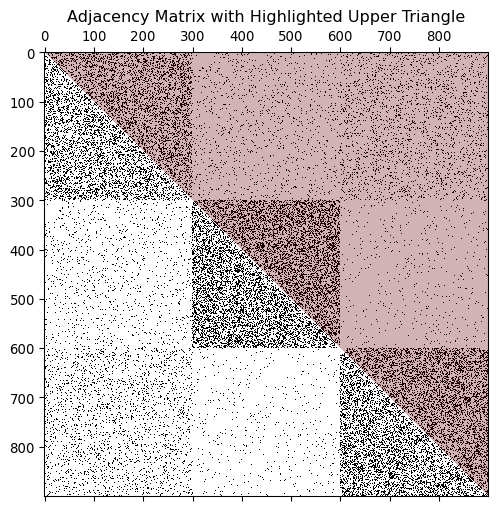
The upper triangle of the adjacency matrix represents i < j over which we take the sum. When c=c' (the diagonal block), we count only the upper half of the block, resulting in \frac{n_c (n_c - 1)}{2}. When c \neq c' (different communities), we count all connections between them, resulting in n_cn_{c'}.
We have now obtaind the likelihood function based only on the community assignment. Maximizing {\cal L} with respect to the community assignment gives us the most likely community assignment for the network.
References
Clauset, Aaron, Mark EJ Newman, and Cristopher Moore. 2004. “Finding Community Structure in Very Large Networks.” Physical Review E—Statistical, Nonlinear, and Soft Matter Physics 70 (6): 066111.
Cohen, Jonathan. 2009. “Graph Twiddling in a Mapreduce World.” Computing in Science & Engineering 11 (4): 29–41.
Fortunato, Santo. 2010. “Community Detection in Graphs.” Physics Reports 486 (3-5): 75–174.
Fortunato, Santo, and Marc Barthelemy. 2007. “Resolution Limit in Community Detection.” Proceedings of the National Academy of Sciences 104 (1): 36–41.
Fortunato, Santo, and Darko Hric. 2016. “Community Detection in Networks: A User Guide.” Physics Reports 659: 1–44.
Goldberg, Andrew V. 1984. “Finding a Maximum Density Subgraph.” Technical Report.
Koujaku, Sadamori, Ichigaku Takigawa, Mineichi Kudo, and Hideyuki Imai. 2016. “Dense Core Model for Cohesive Subgraph Discovery.” Social Networks 44: 143–52.
Luce, R Duncan. 1950. “Connectivity and Generalized Cliques in Sociometric Group Structure.” Psychometrika 15 (2): 169–90.
Mokken, Robert J et al. 1979. “Cliques, Clubs and Clans.” Quality & Quantity 13 (2): 161–73.
Nadakuditi, Raj Rao, and Mark EJ Newman. 2012. “Graph Spectra and the Detectability of Community Structure in Networks.” Physical Review Letters 108 (18): 188701.
Palla, Gergely, Imre Derényi, Illés Farkas, and Tamás Vicsek. 2005. “Uncovering the Overlapping Community Structure of Complex Networks in Nature and Society.” Nature 435 (7043): 814–18.
Peel, Leto, Daniel B Larremore, and Aaron Clauset. 2017. “The Ground Truth about Metadata and Community Detection in Networks.” Science Advances 3 (5): e1602548.
Peixoto, Tiago P. 2019. “Bayesian Stochastic Blockmodeling.” Advances in Network Clustering and Blockmodeling, 289–332.
Saito, Kazumi, Takeshi Yamada, and Kazuhiro Kazama. 2008. “Extracting Communities from Complex Networks by the k-Dense Method.” IEICE Transactions on Fundamentals of Electronics, Communications and Computer Sciences 91 (11): 3304–11.
Seidman, Stephen B. 1983. “Network Structure and Minimum Degree.” Social Networks 5 (3): 269–87.
Seidman, Stephen B, and Brian L Foster. 1978. “A Graph-Theoretic Generalization of the Clique Concept.” Journal of Mathematical Sociology 6 (1): 139–54.
Shi, Jianbo, and Jitendra Malik. 2000. “Normalized Cuts and Image Segmentation.” IEEE Transactions on Pattern Analysis and Machine Intelligence 22 (8): 888–905.
Wang, Nan, Jingbo Zhang, Kian-Lee Tan, and Anthony KH Tung. 2010. “On Triangulation-Based Dense Neighborhood Graph Discovery.” Proceedings of the VLDB Endowment 4 (2): 58–68.