Node Degree: The Building Block of Network Analysis
What you’ll learn in this module
This module introduces a single, powerful idea — the node’s degree — and shows how that simple number reveals a network’s structure and behavior.
You’ll learn:
- What degree and degree distribution mean and how to read them.
- How to visualize degree distributions so underlying patterns become clear.
- The counterintuitive Friendship Paradox and the notion of degree bias.
- Practical consequences for network robustness, spreading processes, and targeted interventions.
1 Node degree
Let’s talk about node degree. A node’s degree is the number of edges touching it. Here we focus on why that simple count matters.
At the level of an individual node, degree measures visibility and influence: high-degree nodes see and can spread information (or infection) quickly; low-degree nodes have limited reach. At the level of a network, the collection of degrees reveals how centralized or evenly distributed connectivity is — and that shape drives many collective behaviors.
The tiny graph above makes the point visually: node A has degree 3 (it connects to three nodes) while B, C, and D each have degree 1. That asymmetry — a mix of hubs and leaves — is common in real networks and underlies many of the phenomena we study.
Degree distribution
Shift your attention from single nodes to the whole network by asking: how common is each degree? The degree distribution answers that question — it lists the fraction of nodes with degree 1, degree 2, degree 3, and so on. Reading this distribution quickly tells you whether connectivity is evenly spread or concentrated in a few nodes.
Why does that summary matter in practice? Because the distribution shapes how networks behave. We have already seen this in the previous modules:
Robustness vs. fragility — Networks with heavy-tailed degree distributions tolerate random node loss (most removals hit low-degree nodes) but are fragile to targeted hub removal, which can fragment the network.
Small-world effects — If a few hubs dominate the degree distribution, they act as shortcuts that dramatically reduce distances between nodes.
We will add an additional interesting example, called the Friendship Paradox, in the next section.
2 The Friendship Paradox
The Friendship Paradox (Scott Feld, 1991) states that your friends have more friends than you do on average. This is not an insult — it is a statistical consequence of how connections are counted in most social networks. This counterintuitive phenomenon emerges from the mathematical properties of networks and has profound implications for how we understand social structures, information flow, and even public health interventions.
At its core, the Friendship Paradox reveals a fundamental asymmetry in social networks: high-degree nodes (popular individuals) are more likely to be counted as friends by others, while low-degree nodes are less likely to be referenced. This creates a sampling bias where the average degree of your friends tends to be higher than your own degree, and indeed higher than the average degree of the entire network.
The network diagram above illustrates the Friendship Paradox with a simple four-node network. The average degree in this network is (1+3+1+1)/4 = 1.5, but when we look at the average degree of each person’s friends, we get a different story.
Let us list all the friendship ties in adjacency list format, along with the degree of each node in parentheses:
- Bob: Alex (1), Carol (1), David (1)
- Alex: Bob (3)
- Carol: Bob (3)
- David: Bob (3)
Now, let’s compute the average degree of a friend.
\frac{\overbrace{1 + 1 + 1}^{\text{Bob's friends}} + \overbrace{3 + 3 + 3}^{\text{The friends of Alex, Carol, and David}}}{\underbrace{6}_{\text{\# of friends}}} = 2
which confirms the friendship paradox, i.e., a someone’s friend tends to have more friends than that someone.
Why this produces the paradox? Notice that high-degree nodes like Bob are referenced multiple times when computing the average degree of a friend. This is because Bob are a friend of many friends! On the other hand, low-degree nodes are referenced less often. This bias towards high-degree nodes is what makes the friendship paradox a paradox.
Beyond a fun trivia, the friendship paradox has practical implications. In social networks, most people will find that their friends have more friends than they do, not because they’re unpopular, but because of this statistical bias. The same principle applies to many other networks: in scientific collaboration networks, your coauthors tend to have more collaborators than you do; in the internet, the websites you link to tend to have more incoming links than your website.
Try it yourself
- Challenge: Can you build a network where your friends always have more friends than you? Test ideas with this interactive Friendship Paradox Game 🎮.
The friendship paradox in public health
This observation has profound practical consequences, especially in public health and epidemiology. To slow an epidemic you can use the friendship paradox to find better targets, called acquaintance immunization (Cohen, Havlin, and ben-Avraham 2003), which goes as follows:
- Pick a random sample of individuals.
- Ask each to nominate one friend.
- Vaccinate the nominated friends (who tend to be better connected).
This works because when people nominate a friend, they’re more likely to name someone with many social connections. By targeting these nominated friends, public health officials can reach the most connected individuals in a network without needing to map the entire social structure.
The acquaintance immunization does not require the knowledge of the entire network structure, which makes it a practical and effective way to slow an epidemic.
Put the idea to the test
Challenge: Can you control an outbreak by vaccinating people chosen via the friendship paradox? Try to outperform random vaccination in this Vaccination Game 🎮.
3 Visualizing degree distributions
The very first step to understand degree distribution is to visualize it. But visualizing degree distribution is not as simple as it seems. Take for example, the following histogram of a degree distribution.
Calculating best minimal value for power law fit
xmin progress: 00%xmin progress: 05%xmin progress: 10%xmin progress: 15%xmin progress: 20%xmin progress: 25%xmin progress: 30%xmin progress: 35%xmin progress: 40%xmin progress: 45%xmin progress: 50%xmin progress: 55%xmin progress: 60%xmin progress: 65%xmin progress: 70%xmin progress: 75%xmin progress: 80%xmin progress: 85%xmin progress: 90%xmin progress: 95%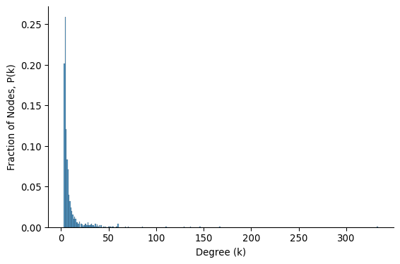
This is a plot you would often see for a real-world network. Most nodes have a very small degree, so they are all crammed into the first few bins on the left. The long tail of high-degree nodes—which hold most edges in the network—is invisible because there are very few of them. This is a fat-tailed distribution, which is a common characteristics of real-world networks.
To solve this, we can plot the same histogram but with both axes on a logarithmic scale. This is called a log–log plot.
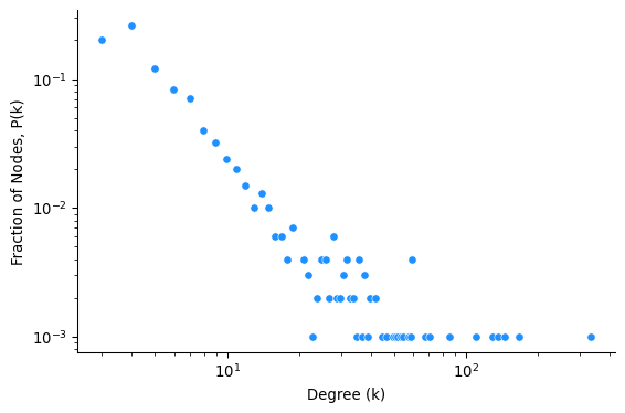
A log–log plot (Figure 4) makes both low- and high-degree nodes visible, revealing heavy-tailed patterns. If the tail is roughly linear, it suggests a power-law degree distribution: the probability a node has degree k falls off as k^{-\gamma}. The slope of the line shows how quickly high-degree nodes become rare. A steeper slope (higher \gamma) means fewer hubs; a shallower slope means more. Interestingly, many real-world networks exhibit power-law(-like) degree distributions, whether they are biological, technical, or social. This universality of power-law degree distributions is one of the foundational insights of Network Science.
Barabási and Albert (1999) (Barabási and Albert 1999) reported the universality of power-law degree distribution in real-world networks. They proposed a mechanism of the emergence of power-law degree distribution, called preferential attachment, which is a subject of a separate module.
Whether power-law degree distribution is a good model for real-world networks is a topic of debate (Artico et al. 2020) (Holme 2019) (Voitalov et al. 2019) (Broido and Clauset 2019). A straight line on a log-log plot is not a unique signature of power-law degree distribution. One can construct it by a mixture of poisson distributions, or some other distributions. Testing whether a network is a power-law or not requires statistical assessment going beyond the visual inspection.
The log-log plot above shows probability density function (PDF) of the degree distribution. It is defined as the fraction of nodes with degree exactly k.
p(k) = \frac{\text{number of nodes with degree } k}{N}
where N is the total number of nodes in the network.
The PDF is useful but often noisy, especially in the tail where there are few observations. A better, more stable choice is the complementary cumulative distribution function (CCDF), which is useful for plotting heavy-tailed distributions.
For a visual comparison of CCDF and PDF, see Figure 3 in (Newman 2005)
\text{CCDF}(k) = P(k' > k) = \sum_{k'=k+1}^\infty p(k')
CCDF represents the fraction of nodes with degree greater than k, or equivalently, the fraction of nodes that survive the degree cutoff k. It is also known as the survival function of the degree distribution.
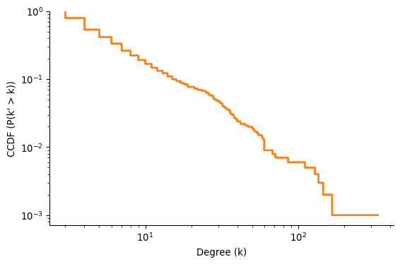
A nice feature of the CCDF compared to the PDF is that it does not require any binning of the data. When calculating the PDF, we need to bin the data into a finite number of bins, which is subject to the choice of bin size. CCDF does not require any binning of the data.
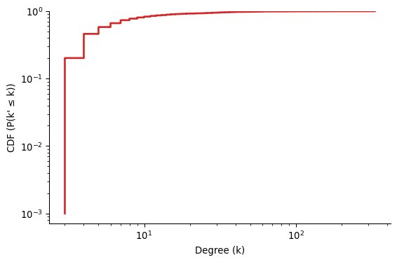
There is a related function called the cumulative distribution function (CDF), which is the fraction of nodes with degree less than or equal to k, i.e., 1 - \text{CCDF}(k).
For degree-heterogenous networks, the CCDF is preferred over the CDF because the CDF does not show the tail of the distribution clearly.
Interpreting the CCDF for Power-Law Distributions
For networks whose degree distribution follows a power law, the CCDF offers a direct path to estimating the power-law exponent, \gamma. Let’s walk through the derivation to see how.
A continuous power-law distribution is defined by the probability density function (PDF): p(k) = Ck^{-\gamma} where C is a normalization constant ensuring the total probability is 1.
The CCDF, which we denote as P(k), is the probability that a node’s degree k' is greater than some value k. We calculate this by integrating the PDF from k to infinity: P(k) = \int_{k}^{\infty} p(k') dk' = \int_{k}^{\infty} Ck'^{-\gamma} dk' Performing the integration gives us: P(k) = C \left[ \frac{k'^{-\gamma+1}}{-\gamma+1} \right]_{k}^{\infty} Assuming \gamma > 1, which is typical for real-world networks, the term k'^{-\gamma+1} approaches zero as k' approaches infinity. The expression simplifies to: P(k) = -C \left( \frac{k^{-\gamma+1}}{-\gamma+1} \right) = \frac{C}{\gamma-1} k^{-(\gamma-1)} This result shows that the CCDF itself follows a power law, P(k) \propto k^{-(\gamma-1)}.
To see what this means for a log-log plot, we take the logarithm of both sides: \log P(k) = \log\left(\frac{C}{\gamma-1}\right) - (\gamma-1)\log(k) This equation is in the form of a straight line, y = b + mx, where:
- y = \log P(k)
- x = \log(k)
- The y-intercept b = \log\left(\frac{C}{\gamma-1}\right)
- The slope m = -(\gamma-1) = 1-\gamma
Key Relationship
For a power-law distribution, the slope of the CCDF on a log-log plot is 1 - \gamma.
This is a crucial point for accurately estimating the scaling exponent from empirical data. For example, if you measure the slope of the CCDF plot to be -1.3, the estimated power-law exponent \gamma is 2.3, not 1.3 (since -1.3 = 1 - 2.3).
References
Artico, Igor, I Smolyarenko, Veronica Vinciotti, and Ernst C Wit. 2020. “How Rare Are Power-Law Networks Really?” Proceedings of the Royal Society A 476 (2241): 20190742.
Barabási, Albert-László, and Réka Albert. 1999. “Emergence of Scaling in Random Networks.” Science 286 (5439): 509–12. https://doi.org/10.1126/science.286.5439.509.
Broido, Anna D., and Aaron Clauset. 2019. “Scale-free networks are rare.” Nature Communications 10 (1). https://doi.org/10.1038/s41467-019-08746-5.
Cohen, Reuven, Shlomo Havlin, and Daniel ben-Avraham. 2003. “Efficient Immunization Strategies for Computer Networks and Populations.” Physical Review Letters 91 (24). https://doi.org/10.1103/physrevlett.91.247901.
Holme, Petter. 2019. “Rare and Everywhere: Perspectives on Scale-Free Networks.” Nature Communications 10 (1): 1016.
Newman, Mark EJ. 2005. “Power Laws, Pareto Distributions and Zipf’s Law.” Contemporary Physics 46 (5): 323–51.
Voitalov, Ivan, Pim Van Der Hoorn, Remco Van Der Hofstad, and Dmitri Krioukov. 2019. “Scale-Free Networks Well Done.” Physical Review Research 1 (3): 033034.