Network Embedding Concepts
1 What is Network Embedding?
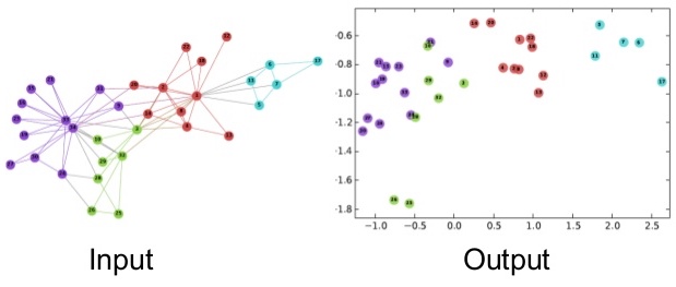
Networks are high-dimensional discrete data that can be difficult to analyze with traditional machine learning methods that assume continuous and smooth data. Network embedding is a technique to represent networks in low-dimensional continuous spaces, enabling us to apply standard machine learning algorithms.
The goal of network embedding is to map each node in a network to a point in a low-dimensional space (typically \mathbb{R}^d where d \ll N) while preserving important structural properties of the network.
2 Exercises
3 Spectral Embedding
Network Compression Approach
Let us approach spectral embedding from the perspective of network compression. Suppose we have an adjacency matrix \mathbf{A} of a network. The adjacency matrix is high-dimensional data, i.e., a matrix of size N \times N for a network of N nodes. We want to compress it into a lower-dimensional matrix \mathbf{U} of size N \times d for a user-defined small integer d < N. A good \mathbf{U} should preserve the network structure and thus can reconstruct the original data \mathbf{A} as closely as possible. This leads to the following optimization problem:
\min_{\mathbf{U}} J(\mathbf{U}),\quad J(\mathbf{U}) = \| \mathbf{A} - \mathbf{U}\mathbf{U}^\top \|_F^2
where:
- \mathbf{U}\mathbf{U}^\top is the outer product of \mathbf{U} and represents the reconstructed network.
- \|\cdot\|_F is the Frobenius norm, which is the sum of the squares of the elements in the matrix.
- J(\mathbf{U}) is the loss function that measures the difference between the original network \mathbf{A} and the reconstructed network \mathbf{U}\mathbf{U}^\top.
By minimizing the Frobenius norm with respect to \mathbf{U}, we obtain the best low-dimensional embedding of the network.
Spectral Decomposition Solution
Consider the spectral decomposition of \mathbf{A}:
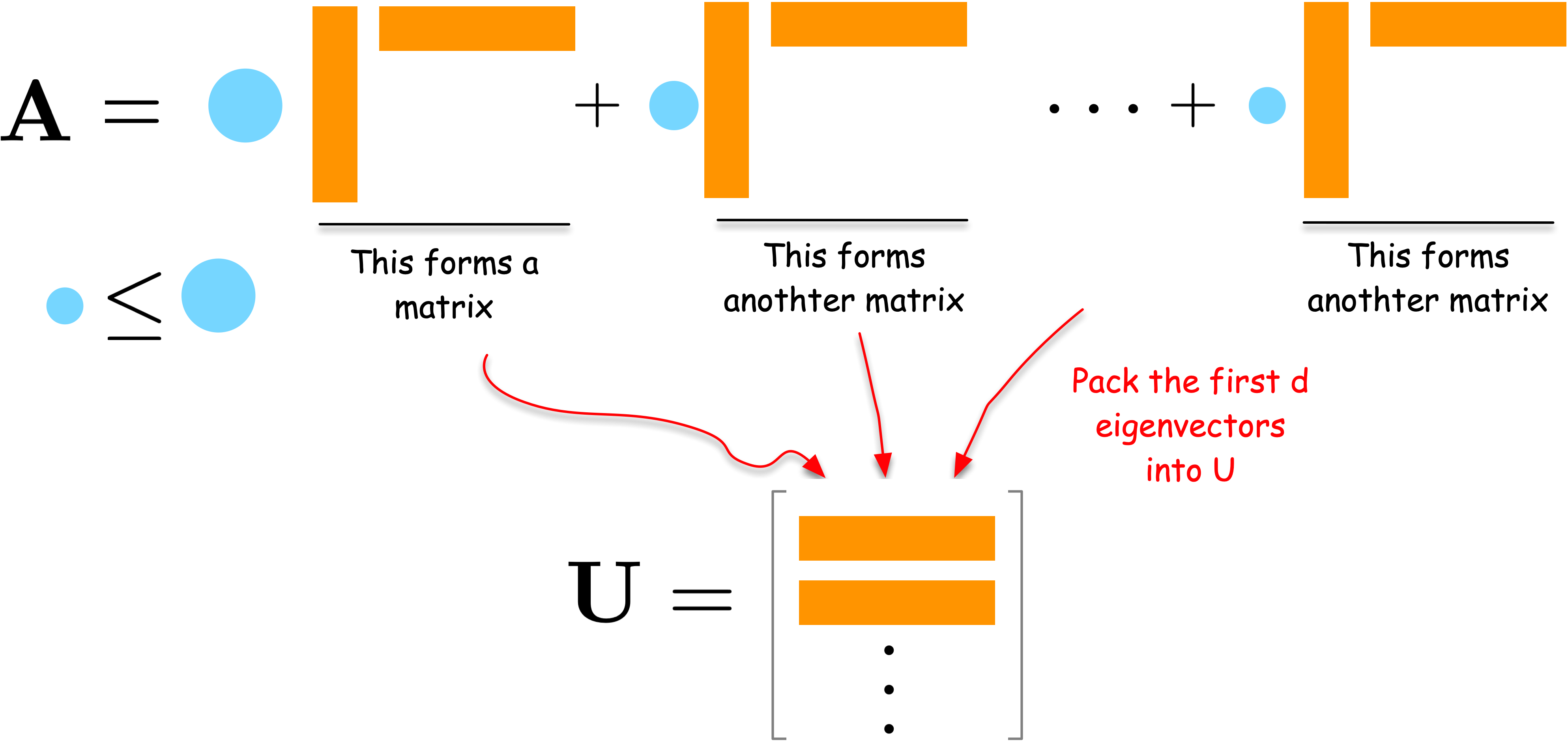
\mathbf{A} = \sum_{i=1}^N \lambda_i \mathbf{u}_i \mathbf{u}_i^\top
where \lambda_i are eigenvalues (weights) and \mathbf{u}_i are eigenvectors. Each term \lambda_i \mathbf{u}_i \mathbf{u}_i^\top is a rank-one matrix that captures a part of the network’s structure. The larger the weight \lambda_i, the more important that term is in describing the network.
To compress the network, we can select the d terms with the largest weights \lambda_i. By combining the corresponding \mathbf{u}_i vectors into a matrix \mathbf{U}, we obtain a good low-dimensional embedding of the network.
For a formal proof, please refer to the Appendix section.
Modularity Embedding
In a similar vein, we can use the modularity matrix to generate a low-dimensional embedding of the network. Let us define the modularity matrix \mathbf{Q} as follows:
Q_{ij} = \frac{1}{2m}A_{ij} - \frac{k_i k_j}{4m^2}
where k_i is the degree of node i, and m is the number of edges in the network.
We then compute the eigenvectors of \mathbf{Q} and use them to embed the network into a low-dimensional space just as we did for the adjacency matrix. The modularity embedding can be used to bipartition the network into two communities using a simple algorithm: group nodes with the same sign of the second eigenvector (Newman 2006).
Laplacian Eigenmap
Laplacian Eigenmap (Belkin and Niyogi 2003) is another approach to compress a network into a low-dimensional space. The fundamental idea behind this method is to position connected nodes close to each other in the low-dimensional space. This approach leads to the following optimization problem:
\min_{\mathbf{U}} J_{LE}(\mathbf{U}),\quad J_{LE}(\mathbf{U}) = \frac{1}{2}\sum_{i,j} A_{ij} \| u_i - u_j \|^2
Derivation steps:
Starting from J_{LE}(\mathbf{U}), we expand:
\begin{aligned} &= \frac{1}{2}\sum_{i,j} A_{ij} \left( \| u_i \|^2 - 2 u_i^\top u_j + \| u_j \|^2 \right) \\ &= \sum_{i} k_i \| u_i \|^2 - \sum_{i,j} A_{ij} u_i^\top u_j\\ &= \sum_{i,j} L_{ij} u_i^\top u_j \end{aligned}
where L_{ij} = k_i if i=j and L_{ij} = -A_{ij} otherwise.
In matrix form: J_{LE}(\mathbf{U}) = \text{Tr}(\mathbf{U}^\top \mathbf{L} \mathbf{U})
See Appendix for full details.
The solution minimizes distances between connected nodes. Through algebraic manipulation (see margin), we can rewrite the objective as J_{LE}(\mathbf{U}) = \text{Tr}(\mathbf{U}^\top \mathbf{L} \mathbf{U}), where \mathbf{L} is the graph Laplacian matrix:
L_{ij} = \begin{cases} k_i & \text{if } i = j \\ -A_{ij} & \text{if } i \neq j \end{cases}
By taking the derivative and setting it to zero:
\frac{\partial J_{LE}}{\partial \mathbf{U}} = 0 \implies \mathbf{L} \mathbf{U} = \lambda \mathbf{U}
Solution: The d eigenvectors associated with the d smallest eigenvalues of the Laplacian matrix \mathbf{L}.
The smallest eigenvalue is always zero (with eigenvector of all ones). In practice, compute d+1 smallest eigenvectors and discard the trivial one.
4 Neural Embedding
Introduction to word2vec
Neural embedding methods leverage neural network architectures to learn node representations. Before discussing graph-specific methods, we first introduce word2vec, which forms the foundation for many neural graph embedding techniques.
word2vec is a neural network model that learns word embeddings in a continuous vector space. It was introduced by Tomas Mikolov and his colleagues at Google in 2013 (Mikolov et al. 2013).
How word2vec Works
word2vec learns word meanings from context, following the linguistic principle: “You shall know a word by the company it keeps” (church1988word?).
This phrase means a person is similar to those they spend time with. It comes from Aesop’s fable The Ass and his Purchaser (500s B.C.): a man brings an ass to his farm on trial. The ass immediately seeks out the laziest, greediest ass in the herd. The man returns the ass, knowing it will be lazy and greedy based on the company it chose.
The Core Idea: Given a target word, predict its surrounding context words within a fixed window. For example, in:
The quick brown fox jumps over a lazy dog
The context of fox (with window size 2) includes: quick, brown, jumps, over.
The window size determines how far we look around the target word. A window size of 2 means we consider 2 words before and 2 words after.
Why This Works: Words appearing in similar contexts get similar embeddings. Consider:
- “The quick brown fox jumps over the fence”
- “The quick brown dog runs over the fence”
- “The student studies in the library”
Both fox and dog appear with words like “quick,” “brown,” and “jumps/runs,” so they’ll have similar embeddings. But student appears in completely different contexts (like “studies,” “library”), so its embedding will be far from fox and dog. This is how word2vec captures semantic similarity without explicit supervision.
Two Training Approaches:
- Skip-gram: Given a target word → predict context words (we’ll use this)
- CBOW: Given context words → predict target word
Skip-gram works better for small datasets and rare words. CBOW is faster to train.
Network Architecture: word2vec uses a simple 3-layer neural network:
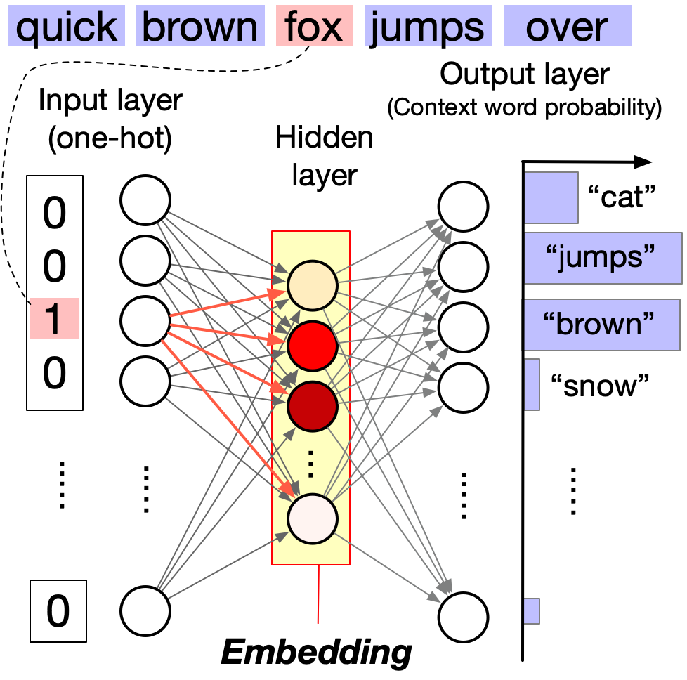
- Input layer (N neurons): One-hot encoding of the target word
- Hidden layer (d neurons, d \ll N): The learned word embedding
- Output layer (N neurons): Probability distribution over context words (via softmax)
The hidden layer activations become the word embeddings—dense, low-dimensional vectors that capture semantic relationships.
For a visual walkthrough of word2vec, see The Illustrated Word2vec by Jay Alammar.
Key Technical Components
The Computational Challenge
To predict context word w_c given target word w_t, we compute:
P(w_c | w_t) = \frac{\exp(\mathbf{v}_{w_c} \cdot \mathbf{v}_{w_t})}{\sum_{w \in V} \exp(\mathbf{v}_w \cdot \mathbf{v}_{w_t})}
This is the softmax function—it converts dot products into probabilities that sum to 1.
The problem: The denominator sums over all vocabulary words (e.g., 100,000+ terms), making training prohibitively slow.
Two Solutions
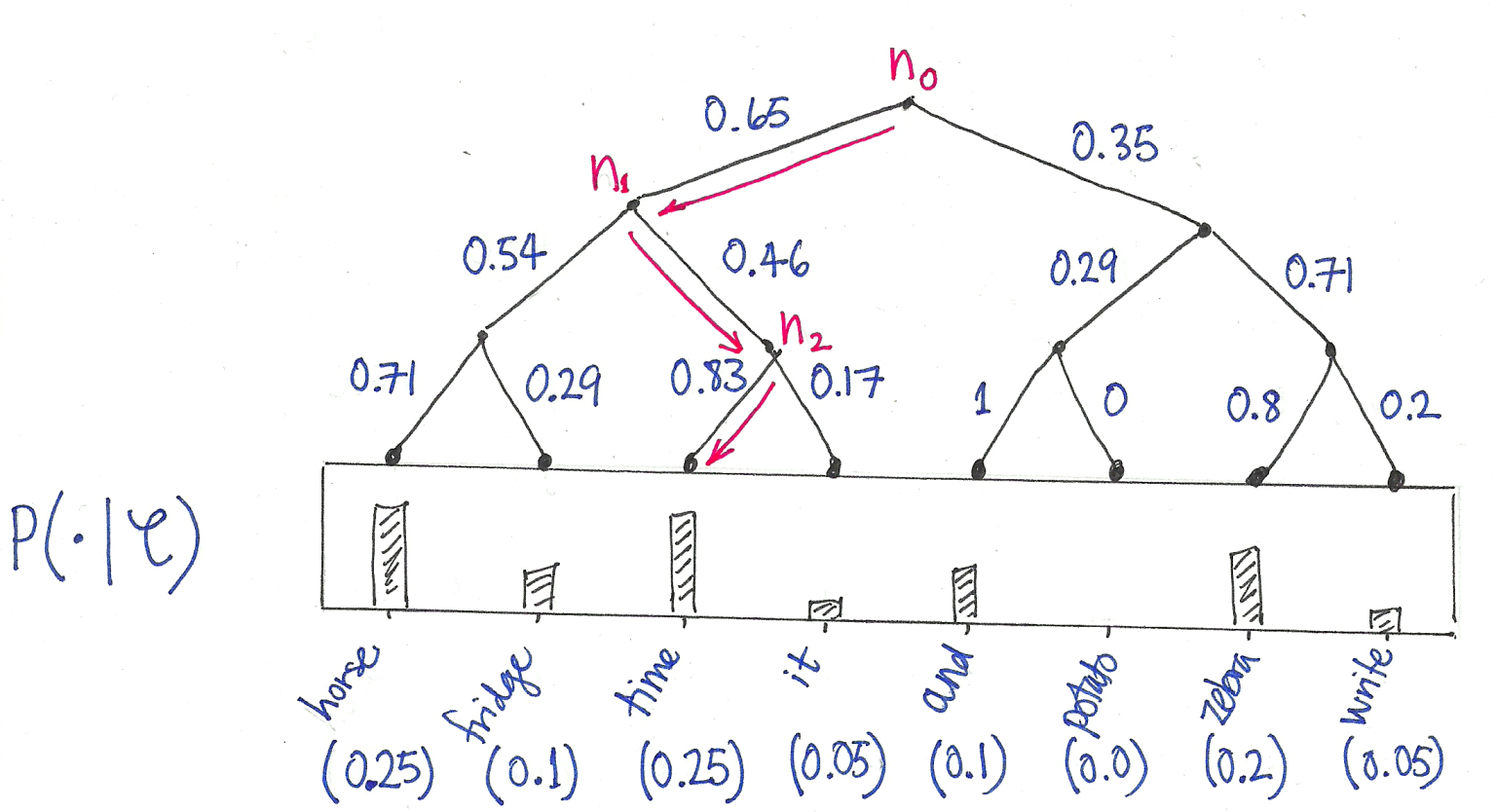
Hierarchical Softmax: Organizes vocabulary as a binary tree with words at leaves. Computing probability becomes traversing root-to-leaf paths, reducing complexity from O(|V|) to O(\log |V|).
Negative Sampling: Instead of normalizing over all words, sample a few “negative” (non-context) words. Contrast the target’s true context with these random words. This approximates the full softmax much more efficiently.
Typically, 5-20 negative samples are enough. The model learns to distinguish true context words from random words.
What’s Special About word2vec?
With word2vec, words are represented as dense vectors, enabling us to explore their relationships using simple linear algebra. This is in contrast to traditional natural language processing (NLP) methods, such as bag-of-words and topic modeling, which represent words as discrete units or high-dimensional vectors.
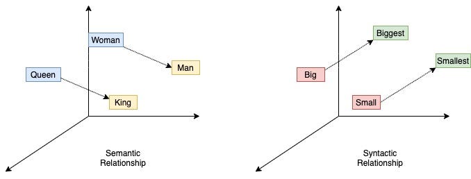
word2vec embeddings can capture semantic relationships, such as analogies (e.g., man is to woman as king is to queen) and can visualize relationships between concepts (e.g., countries and their capitals form parallel vectors in the embedding space).
5 Graph Embedding with word2vec
How can we apply word2vec to graph data? There is a critical challenge: word2vec takes sequences of words as input, while graph data are discrete and unordered. A solution to fill this gap is random walk, which transforms graph data into a sequence of nodes. Once we have a sequence of nodes, we can treat it as a sequence of words and apply word2vec.
Random walks create “sentences” from graphs: each walk is a sequence of nodes, just like a sentence is a sequence of words.
DeepWalk

DeepWalk is one of the pioneering works to apply word2vec to graph data (Perozzi, Al-Rfou, and Skiena 2014). It views the nodes as words and the random walks on the graph as sentences, and applies word2vec to learn the node embeddings.
More specifically, the method contains the following steps:
- Sample multiple random walks from the graph.
- Treat the random walks as sentences and feed them to word2vec to learn the node embeddings.
DeepWalk typically uses the skip-gram model with hierarchical softmax for efficient training.
node2vec
node2vec (Grover and Leskovec 2016) extends DeepWalk with biased random walks controlled by two parameters:
P(v_{t+1} = x | v_t = v, v_{t-1} = t) \propto \begin{cases} \frac{1}{p} & \text{if } d(t,x) = 0 \text{ (return to previous)} \\ 1 & \text{if } d(t,x) = 1 \text{ (close neighbor)} \\ \frac{1}{q} & \text{if } d(t,x) = 2 \text{ (explore further)} \\ \end{cases}
where d(t,x) is the shortest path distance from the previous node t to candidate node x.
Controlling Exploration:
- Low p → return bias (local revisiting)
- Low q → outward bias (exploration)
- High q → inward bias (stay local)
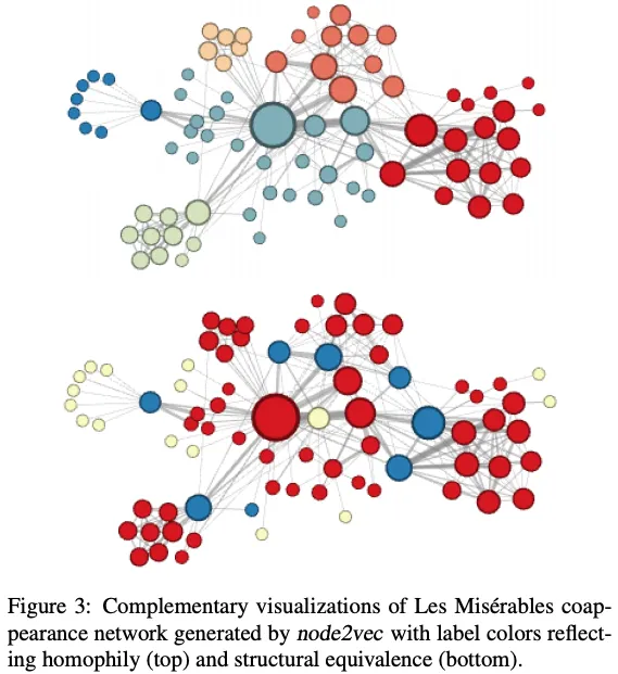
Two Exploration Strategies:

- BFS-like (low q): Explore immediate neighborhoods → captures community structure
- DFS-like (high q): Explore deep paths → captures structural roles
Technical Note: node2vec uses negative sampling instead of hierarchical softmax, which affects embedding characteristics (Kojaku et al. 2021; Dyer 2014).
LINE
LINE (Tang et al. 2015) is another pioneering work to learn node embeddings by directly optimizing the graph structure. It is equivalent to node2vec with p=1, q=1, and window size 1.
Neural methods are less transparent, but recent work establishes equivalences to spectral methods under specific conditions (Qiu et al. 2018; Kojaku et al. 2024). Surprisingly, DeepWalk, node2vec, and LINE are also provably optimal for the stochastic block model (Kojaku et al. 2024).
6 Hyperbolic Embeddings: Beyond Euclidean Space
All the embedding methods we’ve discussed so far operate in Euclidean space (standard flat geometry). However, many real-world networks exhibit hierarchical structures and scale-free properties that are difficult to capture in Euclidean space. Hyperbolic embeddings offer a powerful alternative by embedding networks in hyperbolic geometry—a curved space with negative curvature.
The Popularity-Similarity Framework
The foundation for hyperbolic network embeddings comes from a seminal discovery: real networks grow by optimizing trade-offs between popularity and similarity (Papadopoulos et al. 2012). When analyzing the evolution of the Internet, metabolic networks, and social networks, Papadopoulos et al. found that new connections are not formed simply by preferential attachment to popular nodes. Instead, nodes balance two factors:
- Popularity: Connecting to well-established, highly connected nodes
- Similarity: Connecting to nodes with similar characteristics or interests
This popularity × similarity optimization has a remarkable geometric interpretation: it naturally emerges as optimization in hyperbolic space. In this framework:
- Node popularity maps to radial position (birth time, with older = more central)
- Node similarity maps to angular distance on a circle
- New connections form to nodes that are hyperbolically closest
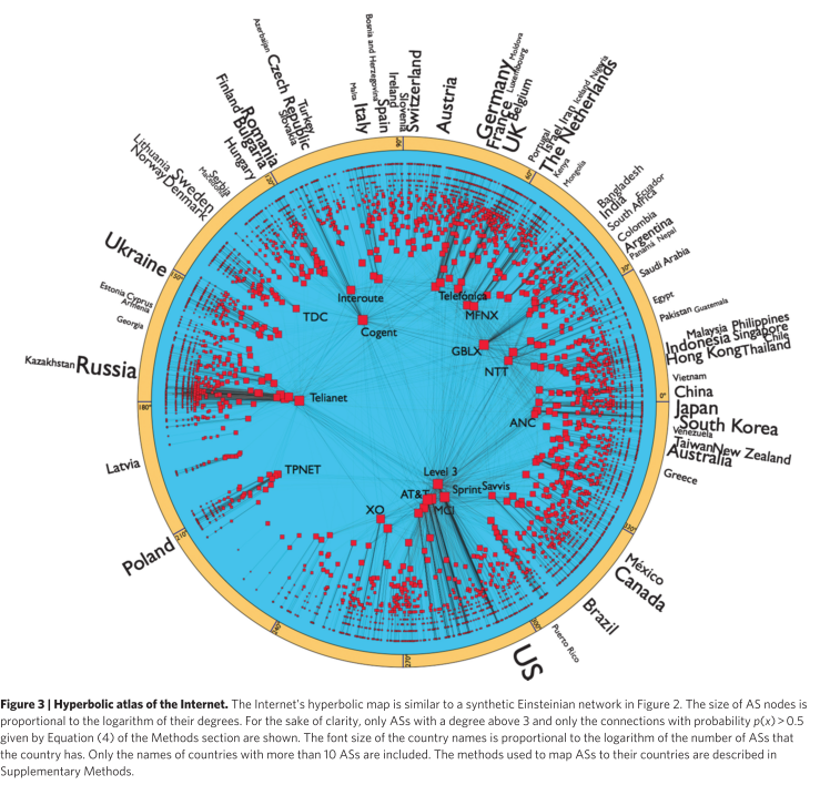
In the popularity-similarity model, hyperbolic distance x_{ij} \approx r_i + r_j + \ln(\theta_{ij}/2) combines popularity (radial coordinates r) and similarity (angular distance \theta). New nodes connect to the m hyperbolically closest nodes.
This framework elegantly explains why preferential attachment emerges as a phenomenon: it’s not a primitive mechanism, but rather a consequence of local geometric optimization. The probability that a node of degree k attracts a new link follows \Pi(k) \propto k, exactly as in preferential attachment—but now with crucial differences in which specific nodes get connected based on their similarity.
The popularity-similarity framework directly validates against real network evolution: the probability of new connections as a function of hyperbolic distance matches theoretical predictions for Internet, metabolic, and social networks, while pure preferential attachment is off by orders of magnitude (Papadopoulos et al. 2012).
Why Hyperbolic Space?
The study of hyperbolic geometry in complex networks emerged from foundational work showing that networks with heterogeneous degree distributions and strong clustering have an effective hyperbolic geometry underneath (Krioukov et al. 2010). Hyperbolic space has a unique property: its volume grows exponentially with radius, similar to how tree-like hierarchies grow. This naturally captures key network properties:
- Scale-free degree distributions: Power-law degrees emerge from negative curvature
- Strong clustering: Nodes form tight communities based on metric proximity
- Small-world property: Short paths exist despite high clustering
- Self-similarity and navigability: Arise from underlying hyperbolic geometry (Serrano, Krioukov, and Boguñá 2008; Boguñá, Krioukov, and Claffy 2009)
The connection between hyperbolic geometry and network structure was established through a series of papers by Krioukov, Boguñá, and colleagues (2008-2010), showing that the statistical mechanics of complex networks maps directly to geometric properties of hyperbolic space.
Mathematical Models of Hyperbolic Space
Hyperbolic space can be represented through different mathematical models, each with different computational properties:
Poincaré Ball Model: Points lie within the unit ball \mathcal{B}^n = \{\mathbf{x} \in \mathbb{R}^n : \|\mathbf{x}\| < 1\}. The distance between two points \mathbf{u}, \mathbf{v} \in \mathcal{B}^n is:
d_P(\mathbf{u}, \mathbf{v}) = \text{arcosh}\left(1 + 2\frac{\|\mathbf{u} - \mathbf{v}\|^2}{(1 - \|\mathbf{u}\|^2)(1 - \|\mathbf{v}\|^2)}\right)

The Poincaré disk (2D version of the ball) visualizes hyperbolic space within a circle. Although shapes appear to shrink near the boundary in Euclidean terms, they are actually all the same size in hyperbolic geometry—the disk has infinite hyperbolic area. Geodesics (shortest paths) appear as circular arcs perpendicular to the boundary. This model is intuitive for visualization but requires careful handling of Riemannian gradients during optimization.
Lorentzian (Hyperboloid) Model: Points lie on the hyperboloid \mathcal{H}^n = \{\mathbf{x} \in \mathbb{R}^{n+1} : \langle\mathbf{x}, \mathbf{x}\rangle_L = -1, x_0 > 0\} where the Lorentzian inner product is:
\langle\mathbf{x}, \mathbf{y}\rangle_L = -x_0 y_0 + x_1 y_1 + \cdots + x_n y_n
The distance between two points \mathbf{u}, \mathbf{v} \in \mathcal{H}^n is:
d_L(\mathbf{u}, \mathbf{v}) = \text{arcosh}(-\langle\mathbf{u}, \mathbf{v}\rangle_L)
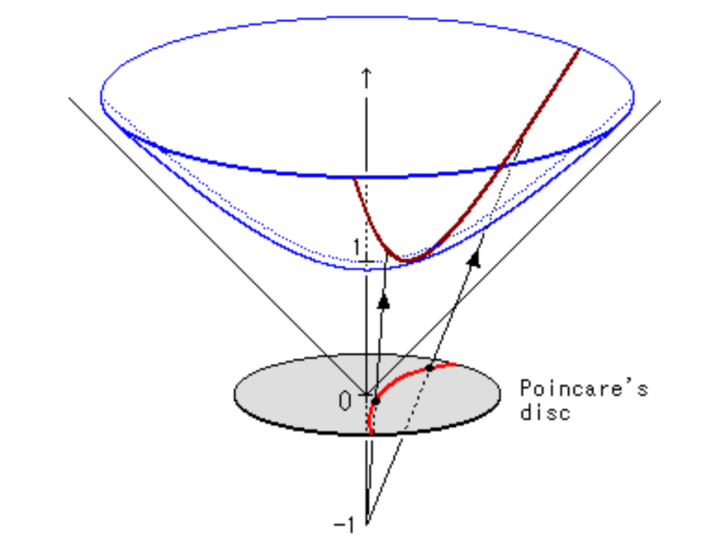
The hyperboloid model embeds hyperbolic space as a sheet in Minkowski space (the geometry of special relativity). Points on the hyperboloid can be projected onto the Poincaré disk, showing the equivalence between models. The Lorentzian model enables more efficient optimization because gradients can be computed in the ambient Euclidean space \mathbb{R}^{n+1}, avoiding complex Riemannian operations.
These models are isometric (distance-preserving transformations exist between them), but differ in computational efficiency. The Poincaré model (Nickel and Kiela 2017) is intuitive but requires complex Riemannian optimization. The Lorentzian model (Nickel and Kiela 2018) trades geometric purity for efficiency by computing gradients in ambient Euclidean space, making hyperbolic embeddings practical for large networks.
