Appendix: The Algebra Behind Modularity and the Block Model
Two derivations the main text quotes but does not carry out. Neither is needed to use the methods; both are worth seeing once.
Why the two forms of modularity are the same
The main text builds modularity as “matches minus chance matches”:
\begin{align} Q &=\frac{1}{2m} \sum_{i=1}^n \sum_{j=1}^n A_{ij} \delta(c_i,c_j) - \sum_{c=1}^C \left( \frac{1}{2m}\sum_{i=1}^n k_i \delta(c, c_i) \right)^2 \end{align}
and then states the standard expression without proof:
Q =\frac{1}{2m} \sum_{i=1}^n \sum_{j=1}^n \left[ A_{ij} - \frac{k_ik_j}{2m} \right]\delta(c_i,c_j)
Here is the path from one to the other.
Start with the first form and factor \frac{1}{2m} out of both terms:
Q =\frac{1}{2m} \left[ \sum_{i=1}^n \sum_{j=1}^n A_{ij} \delta(c_i,c_j) - \frac{1}{2m}\sum_{c=1}^C \left( \sum_{i=1}^n k_i \delta(c, c_i) \right)^2 \right]
Now use (\sum_i a_i)^2 = (\sum_i a_i)( \sum_j a_j) to expand the squared term. The second copy of the sum gets a fresh index j:
Q =\frac{1}{2m} \left[ \sum_{i=1}^n \sum_{j=1}^n A_{ij} \delta(c_i,c_j) - \frac{1}{2m}\sum_{c=1}^C \left( \sum_{i=1}^n k_i \delta(c, c_i) \right) \left( \sum_{j=1}^n k_j \delta(c, c_j) \right)\right]
Two independent sums multiplied together are one double sum, (\sum_i a_i)( \sum_j a_j) = \sum_i \sum_j a_ia_j:
Q =\frac{1}{2m} \left[ \sum_{i=1}^n \sum_{j=1}^n A_{ij} \delta(c_i,c_j) - \frac{1}{2m}\sum_{c=1}^C \left( \sum_{i=1}^n \sum_{j=1}^n k_i k_j \delta(c, c_i) \delta(c, c_j) \right)\right]
The last step is the one that does the work. Summing \delta(c,c_i)\delta(c,c_j) over every color c gives 1 exactly when i and j have the same color and 0 otherwise — which is what \delta(c_i,c_j) means. So the outer sum over c disappears:
Q =\frac{1}{2m} \left[ \sum_{i=1}^n \sum_{j=1}^n A_{ij} \delta(c_i,c_j) - \frac{1}{2m} \sum_{i=1}^n \sum_{j=1}^n k_i k_j \delta(c_i,c_j) \right]
Collect the common factors and the standard form falls out:
Q =\frac{1}{2m} \sum_{i=1}^n \sum_{j=1}^n \left[ A_{ij} - \frac{k_ik_j}{2m} \right]\delta(c_i,c_j)
Read the bracket as the payoff of a single pair: the edge you observe, minus the k_ik_j/2m edges the configuration model expects between two nodes of degree k_i and k_j. Modularity is that surplus, summed over every pair in the same community.
Fitting the stochastic block model
The main text states the answer — the estimated edge probability between two blocks is the number of edges you see divided by the number of pairs that could have carried one. Here is the maximum-likelihood argument behind it.
Setup
Under the SBM, each pair of nodes gets an independent coin flip whose bias depends only on the two communities involved, P(A_{ij}=1 \mid c_i, c_j) = p_{c_ic_j}. The probability of the whole observed network, given an assignment \{c_i\}, is the product of those flips over the i<j pairs:
P(\left\{A_{ij}\right\} \mid \left\{c_i\right\}) = \prod_{i<j} p_{c_i c_j}^{\,A_{ij}} \left(1-p_{c_i c_j}\right)^{1-A_{ij}}
Taking the logarithm turns the product into a sum, which is why nobody ever maximizes a likelihood directly:
{\cal L} = \sum_{i<j} \left[ A_{ij} \log p_{c_ic_j} + (1-A_{ij}) \log (1-p_{c_ic_j}) \right]
Why setting the derivative to zero is enough
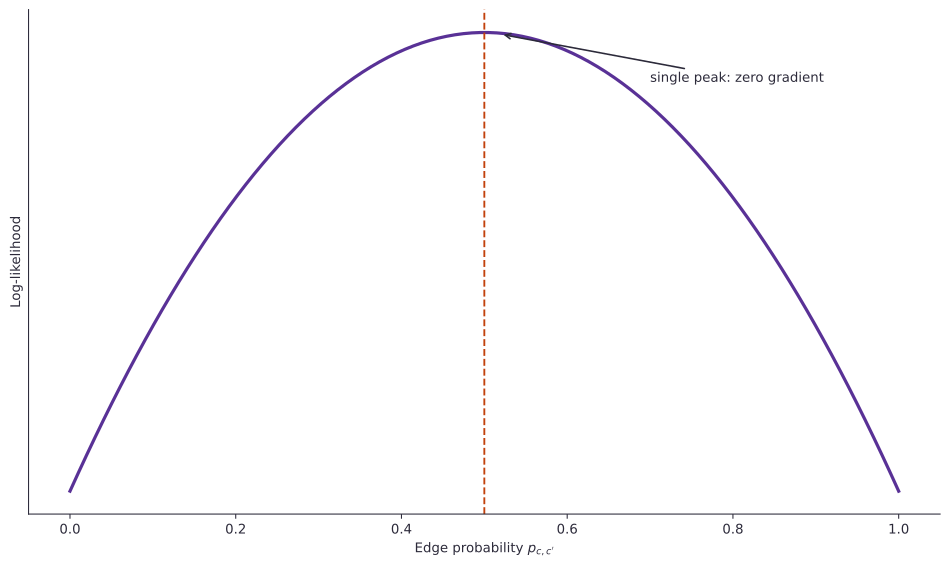
Hold the community assignment fixed and treat {\cal L} as a function of one block probability p_{cc'}. Each term is either \log p or \log(1-p), both of which are concave, and a sum of concave functions is concave. So {\cal L} is a hill with a single peak in p_{cc'}: find the one place where the slope is zero and you have found the maximum, with no risk of a false summit.
Taking the derivative
Differentiate {\cal L} with respect to p_{cc'} for c \neq c'. Only the pairs with one endpoint in c and the other in c' survive, and the indicator \delta(c_i,c)\delta(c_j,c') + \delta(c_i,c')\delta(c_j,c) picks them out in either order:
\frac{\partial {\cal L}}{\partial p_{cc'}} = \sum_{i<j} \left[ \frac{A_{ij}}{p_{cc'}} - \frac{1-A_{ij}}{1-p_{cc'}} \right] \left[ \delta(c_i,c)\delta(c_j,c') + \delta(c_i,c')\delta(c_j,c) \right]
Write m_{cc'} for the number of edges between the two blocks and N_{cc'} for the number of pairs between them. The first sum collects the edges, the second collects the non-edges, of which there are N_{cc'} - m_{cc'}:
\frac{\partial {\cal L}}{\partial p_{cc'}} = \frac{m_{cc'}}{p_{cc'}} - \frac{N_{cc'} - m_{cc'}}{1-p_{cc'}}
Note the numerator of the second term. It is the count of pairs that are not edges, not the count of pairs — a step that is easy to drop and that changes the answer. Setting the derivative to zero:
m_{cc'}(1-p_{cc'}) = (N_{cc'} - m_{cc'})\, p_{cc'} \quad\Longrightarrow\quad \widehat{p}_{cc'} = \frac{m_{cc'}}{N_{cc'}}
Counting the pairs
All that remains is N_{cc'}, the number of node pairs with one endpoint in block c and the other in block c':
N_{cc'} = \sum_{i < j} \delta(c_i,c)\delta(c_j,c') + \delta(c_i,c')\delta(c_j,c) = \begin{cases} n_cn_{c'} & \text{if } c \neq c' \\[4pt] \dfrac{n_c (n_c - 1)}{2} & \text{if } c = c' \end{cases}
The two cases come from summing over i<j only, which is the upper triangle of the adjacency matrix.
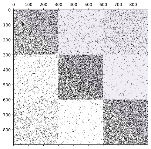
For an off-diagonal block the n_c \times n_{c'} rectangle lies wholly inside the upper triangle, so every one of its n_c n_{c'} pairs is counted once. For a diagonal block the n_c \times n_c square straddles the diagonal, so only the half above it counts: n_c(n_c-1)/2 pairs.
What this does not give you
Everything above assumes the community assignment is already known. The estimate \widehat{p}_{cc'} = m_{cc'}/N_{cc'} tells you the best block probabilities for that assignment, and substituting it back into {\cal L} gives a score for the assignment itself. Maximizing that score over assignments is the actual problem, it is not concave, and it is intractable — the same wall modularity maximization runs into. See the main text for what practitioners do about it.