Appendix: Why the Second Eigenvalue Sets the Clock
The main text claimed one thing without proof: the speed at which a random walk forgets its starting point is governed by the second largest eigenvalue of the transition matrix. This appendix earns that claim. It assumes you have met eigenvalues and eigenvectors before; if you have not, the result in the concepts page is all you need to use random walks in practice.
The Obstacle: The Transition Matrix Is Not Symmetric
The short-term behavior of a random walk is
x(t) = x(0)\,\mathbf{P}^t ,
so everything hinges on computing a high power of a matrix. That is easy when a matrix splits as \mathbf{Q}\mathbf{\Lambda}\mathbf{Q}^{-1}, because then the power falls onto the diagonal alone: \mathbf{Q}\mathbf{\Lambda}^t\mathbf{Q}^{-1}.
The obstacle is that \mathbf{P} = \mathbf{D}^{-1}\mathbf{A} is not symmetric — dividing each row by a different degree destroys the symmetry of \mathbf{A} — so we cannot simply reach for the eigendecomposition of a symmetric matrix, which is the one case that is guaranteed to behave well.
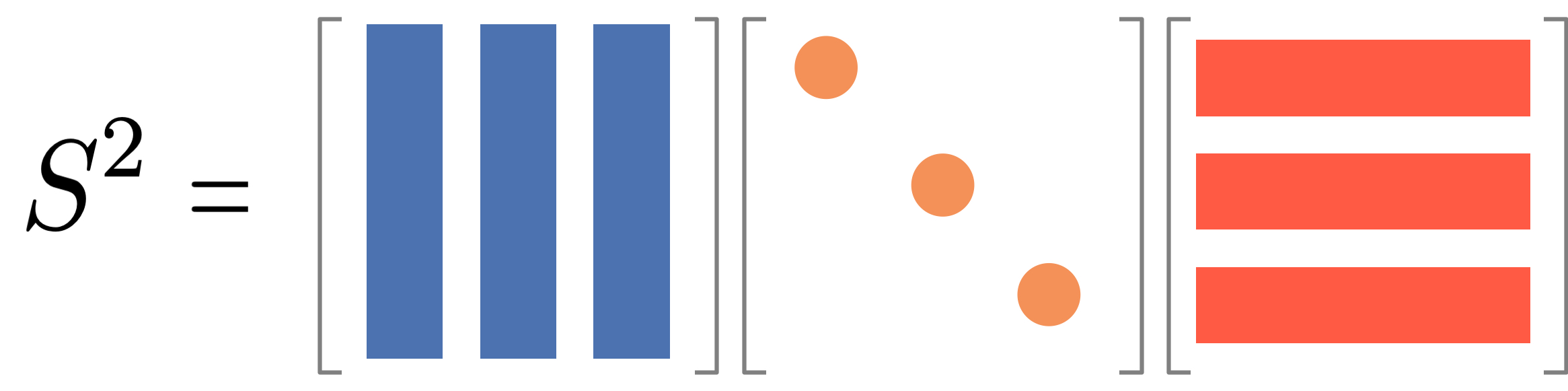
Any symmetric real matrix is diagonalizable with an orthogonal \mathbf{Q} (that is, \mathbf{Q}\mathbf{Q}^\top = \mathbf{I}). A general matrix may be diagonalizable, but its \mathbf{Q} need not be orthogonal — which is exactly the property the argument below needs.
The Trick: Move Half a Degree to Each Side
The way around it is to move the degrees around until what remains is symmetric. Split \mathbf{D}^{-1} into two halves and put one on each side:
\mathbf{P} = \mathbf{D}^{-1}\mathbf{A} = \mathbf{D}^{-\frac{1}{2}} \underbrace{\left( \mathbf{D}^{-\frac{1}{2}} \mathbf{A} \mathbf{D}^{-\frac{1}{2}} \right)}_{\overline{\mathbf{A}}} \mathbf{D}^{\frac{1}{2}}
that is,
\mathbf{P} = \mathbf{D}^{-\frac{1}{2}} \overline{\mathbf{A}} \mathbf{D}^{\frac{1}{2}} .
The two ingredients are:
- Diagonal degree matrix \mathbf{D}: the diagonal matrix whose entries are the node degrees,
\mathbf{D} = \begin{pmatrix} k_1 & 0 & \cdots & 0 \\ 0 & k_2 & \cdots & 0 \\ \vdots & \vdots & \ddots & \vdots \\ 0 & 0 & \cdots & k_N \end{pmatrix}
- Normalized adjacency matrix \overline{\mathbf{A}}: each entry of \mathbf{A} divided by the square roots of the two degrees at its ends,
\overline{\mathbf{A}} = \mathbf{D}^{-\frac{1}{2}} \mathbf{A} \mathbf{D}^{-\frac{1}{2}}, \qquad \overline{A}_{ij} = \frac{A_{ij}}{\sqrt{k_i k_j}} .
Because \mathbf{A} is symmetric for an undirected network and the same factor is applied on both sides, \overline{\mathbf{A}} is symmetric too. That is the whole point of the manoeuvre, and it is the algebraic face of the reversibility we established in the main text: a walk that looks the same played backwards has a transition matrix that is a symmetric matrix in disguise.
Diagonalizing the Disguise
Being symmetric, \overline{\mathbf{A}} has an orthogonal eigendecomposition
\overline{\mathbf{A}} = \mathbf{Q} \mathbf{\Lambda} \mathbf{Q}^\top, \qquad \mathbf{Q}\mathbf{Q}^\top = \mathbf{I},
with \mathbf{\Lambda} diagonal and real. Substituting into the previous identity gives
\mathbf{P} = \mathbf{Q}_L \mathbf{\Lambda} \mathbf{Q}_R^\top, \qquad \mathbf{Q}_L = \mathbf{D}^{-\frac{1}{2}} \mathbf{Q}, \quad \mathbf{Q}_R = \mathbf{D}^{\frac{1}{2}} \mathbf{Q} .
So \mathbf{P} has the same eigenvalues as \overline{\mathbf{A}}; only the eigenvectors are reweighted by degree. And \mathbf{Q}_L, \mathbf{Q}_R are built so that
\mathbf{Q}_R^\top \mathbf{Q}_L = \mathbf{Q}^\top \mathbf{D}^{\frac{1}{2}} \mathbf{D}^{-\frac{1}{2}} \mathbf{Q} = \mathbf{Q}^\top \mathbf{Q} = \mathbf{I},
which is what makes powers collapse. For t = 2,
\begin{aligned} \mathbf{P}^2 & = \mathbf{Q}_L \mathbf{\Lambda} \underbrace{\mathbf{Q}_R^\top \mathbf{Q}_L}_{= \mathbf{I}} \mathbf{\Lambda} \mathbf{Q}_R^\top \\ & = \mathbf{Q}_L \mathbf{\Lambda}^2 \mathbf{Q}_R^\top , \end{aligned}
and by induction, for every t,
\mathbf{P}^t = \mathbf{Q}_L \mathbf{\Lambda}^t \mathbf{Q}_R^\top .

Reading the Decomposition One Mode at a Time
Write q_L^{(\ell)} for the \ell-th column of \mathbf{Q}_L and q_R^{(\ell)} for the \ell-th column of \mathbf{Q}_R. Then
x(t) = x(0)\,\mathbf{P}^t = \sum_{\ell=1}^{N} \lambda_\ell^{\,t}\, \left( x(0)\cdot q_L^{(\ell)} \right) \left( q_R^{(\ell)} \right)^\top .
The walk is a sum of N modes. Each mode is a fixed pattern q_R^{(\ell)} over the nodes, present in the initial condition with weight x(0)\cdot q_L^{(\ell)}, and multiplied by \lambda_\ell at every step.
The first mode is the stationary distribution. Order the eigenvalues 1 = \lambda_1 > \lambda_2 \geq \cdots \geq \lambda_N > -1. Check that \mathbf{D}^{1/2}\mathbf{1} is an eigenvector of \overline{\mathbf{A}} with eigenvalue 1:
\overline{\mathbf{A}}\, \mathbf{D}^{\frac{1}{2}}\mathbf{1} = \mathbf{D}^{-\frac{1}{2}} \mathbf{A} \mathbf{1} = \mathbf{D}^{-\frac{1}{2}} \mathbf{k} = \mathbf{D}^{\frac{1}{2}}\mathbf{1},
using \mathbf{A}\mathbf{1} = \mathbf{k}, the vector of degrees. Normalising it to unit length gives q^{(1)} = \mathbf{D}^{1/2}\mathbf{1}/\sqrt{2m}, since \|\mathbf{D}^{1/2}\mathbf{1}\|^2 = \sum_i k_i = 2m. Therefore
q_L^{(1)} = \mathbf{D}^{-\frac{1}{2}} q^{(1)} = \frac{\mathbf{1}}{\sqrt{2m}}, \qquad q_R^{(1)} = \mathbf{D}^{\frac{1}{2}} q^{(1)} = \frac{\mathbf{k}}{\sqrt{2m}} .
The first mode’s weight is x(0)\cdot q_L^{(1)} = \frac{1}{\sqrt{2m}}\sum_i x_i(0) = \frac{1}{\sqrt{2m}} for any starting distribution, because probabilities sum to 1. So the \ell=1 term of the sum is
1^{\,t}\cdot \frac{1}{\sqrt{2m}} \cdot \frac{\mathbf{k}^\top}{\sqrt{2m}} = \frac{\mathbf{k}^\top}{2m} = \boldsymbol{\pi} ,
which is the \pi_i = k_i/2m of the main text, recovered spectrally, and it does not depend on x(0) at all.
Everything else decays. For \ell \geq 2 we have |\lambda_\ell| < 1, so \lambda_\ell^{\,t} \to 0. Hence
x(t) - \boldsymbol{\pi} = \sum_{\ell \geq 2} \lambda_\ell^{\,t}\, \left( x(0)\cdot q_L^{(\ell)} \right)\left( q_R^{(\ell)} \right)^\top,
and for large t the sum is dominated by the slowest-decaying term, the one with the largest |\lambda_\ell| among \ell \geq 2. The error therefore behaves like \lambda_2^{\,t} = e^{-t/\tau} with
\tau = \frac{1}{-\log \lambda_2} \approx \frac{1}{1-\lambda_2} \quad \text{for } \lambda_2 \text{ close to } 1 .
This is the relaxation time of the main text, and it is why the spectral gap 1 - \lambda_2 is the number to look at.
From Decay Rate to Mixing Time
Mixing time was defined with the \ell_1 distance,
t_{\text{mix}} = \min\left\{t : \max_{x(0)} \|x(t) - \boldsymbol{\pi}\|_{1} \leq \epsilon\right\}, \qquad \|x(t) - \boldsymbol{\pi}\|_1 = \sum_i |x_i(t) - \pi_i| .
Converting the mode-by-mode decay above into a bound on this sum costs one Cauchy–Schwarz step and one factor accounting for the smallest stationary probability. For a reversible walk the standard result is
t_{\text{mix}} < \frac{1}{1-\lambda_\star} \log\left( \frac{1}{\epsilon\, \min_i \pi_i} \right), \qquad \lambda_\star = \max\left(|\lambda_2|,\ |\lambda_N|\right) .
Two things to notice. First, the relevant quantity is the largest eigenvalue in magnitude other than 1: a walk can be slow because \lambda_2 is near +1 (a bottleneck) or because \lambda_N is near -1 (near-periodicity, as in a nearly bipartite network). A lazy walk, which stays put with probability 1/2, kills the second failure mode outright. Second, \tau = 1/(1-\lambda_2) by itself is a time scale, not a bound: the logarithm says how many multiples of \tau you need, and it grows as you demand a tighter \epsilon or as the rarest node becomes rarer.
The normalized Laplacian is \overline{\mathbf{L}} = \mathbf{I} - \overline{\mathbf{A}}, so its eigenvalues are exactly 1 - \lambda_\ell and its second smallest is the spectral gap \mu = 1 - \lambda_2. Everything above can therefore be rewritten in Laplacian language without changing a single number.
Worked Numbers
Two ten-node networks, so the arithmetic is checkable by hand or in three lines of numpy.
| Network | \lambda_2 | gap 1-\lambda_2 | \tau |
|---|---|---|---|
| Two 5-cliques joined by one edge | 0.927 | 0.073 | \approx 14 |
| One 10-clique | -1/9 \approx -0.111 | 1.111 | \approx 0.9 |
Same node count, same walk rule. The single bottleneck edge multiplies the relaxation time by about fifteen. Removing the bottleneck — merging the cliques — makes the walk mix in essentially one step, because from any node in a clique every other node is one step away.
For the complete graph K_N the eigenvalues can be written down exactly: \mathbf{P} = (\mathbf{J} - \mathbf{I})/(N-1), whose eigenvalues are 1 (once) and -1/(N-1) (N-1 times). For N = 10 that is -1/9, matching the table.