Teaching computers how to understand words#
Imagine trying to explain the meaning of words to someone who only understands numbers. This is exactly the challenge we face when teaching computers to process text. Just as we need to translate between languages, we need to translate between the world of human language and the world of computer numbers. This translation process has evolved dramatically over time, becoming increasingly sophisticated in its ability to capture the nuances of meaning.
One-Hot Encoding: The First Step#
The simplest approach to this translation challenge is one-hot encoding, akin to giving each word its own unique light switch in a vast room of switches. When representing a word, we turn on its switch and leave all others off. For example, in a tiny vocabulary of just three words {cat, dog, fish}:
‘cat’ becomes [1, 0, 0]
‘dog’ becomes [0, 1, 0]
‘fish’ becomes [0, 0, 1]
While simple, this approach has a fundamental flaw: it suggests that all words are equally different from each other. In this representation, ‘cat’ is just as different from ‘dog’ as it is from ‘algorithm’ - something we know isn’t true in real language use.
Distributional Hypothesis#
What is missing in one-hot encoding is the notion of context.
One associates cat with dog because they have similar context, while cat is more different from fish than dog because they are in different contexts.
This is the core idea of the distributional hypothesis.
In a nutshell, the distributional hypothesis states that:
Words that frequently appear together in text (co-occur) are likely to be semantically related
The meaning of a word can be inferred by examining the distribution of other words around it
Similar words will have similar distributions of surrounding context words
This hypothesis forms the theoretical foundation for many modern word embedding techniques.
Note
The idea that words can be understood by their context is captured by the famous linguistic principle: “You shall know a word by the company it keeps” [1]. This principle suggests that the meaning of a word is not inherent to the word itself, but rather emerges from how it is used alongside other words.
Tip
The ancient Buddhist concept of Apoha, developed by Dignāga in the 5th-6th century CE, shares similarities with modern distributional semantics. According to Apoha theory, we understand concepts by distinguishing what they are not - for example, we know what a “cow” is by recognizing everything that is not a cow. This mirrors how modern word embeddings define words through their relationships and contrasts with other words, showing how both ancient philosophy and contemporary linguistics recognize that meaning emerges from relationships between concepts.

TF-IDF: A Simple but Powerful Word Embedding Technique#
Distributional Hypothesis#
What is missing in one-hot encoding is the notion of context. One associates cat with dog because they have similar context, while cat is more different from fish than dog because they are in different contexts. This is the core idea of the distributional hypothesis.
In a nutshell, the distributional hypothesis states that we can understand the meaning of a word by examining the context in which it appears. Just as you might understand a person by the company they keep, we can understand a word by the words that surround it. This principle suggests that words appearing in similar contexts likely have similar meanings.
Note
The idea that words can be understood by their context is captured by the famous linguistic principle: “You shall know a word by the company it keeps” [1]. This principle suggests that the meaning of a word is not inherent to the word itself, but rather emerges from how it is used alongside other words.
TF-IDF: Words as Patterns of Usage#
The distributional hypothesis leads us to an important question: How can we capture these contextual patterns mathematically? More specifically, what is a good unit of “context”? A natural choice is to let the document be the unit of context. The distributional hypothesis suggests that words that frequently appear in the same documents are likely to be semantically related.
First Attempt: Word-Document Count Matrix#
Let’s try to organize this information systematically. Imagine creating a giant table where:
Each row represents a word
Each column represents a document
Each cell contains the count of how often that word appears in that document
from sklearn.feature_extraction.text import CountVectorizer
import numpy as np
import pandas as pd

# Sample documents
documents = [
    "The cat chases mice in the garden",
    "The dog chases cats in the park",
    "Mice eat cheese in the house",
    "The cat and dog play in the garden"
]

# Create word count matrix
vectorizer = CountVectorizer()
count_matrix = vectorizer.fit_transform(documents)
words = vectorizer.get_feature_names_out()

# Display as a table
df = pd.DataFrame(count_matrix.toarray(), columns=words)
df.style.background_gradient(cmap='cividis', axis = None).set_caption("Word-Document Count Matrix")
| and | cat | cats | chases | cheese | dog | eat | garden | house | in | mice | park | play | the | |
|---|---|---|---|---|---|---|---|---|---|---|---|---|---|---|
| 0 | 0 | 1 | 0 | 1 | 0 | 0 | 0 | 1 | 0 | 1 | 1 | 0 | 0 | 2 |
| 1 | 0 | 0 | 1 | 1 | 0 | 1 | 0 | 0 | 0 | 1 | 0 | 1 | 0 | 2 |
| 2 | 0 | 0 | 0 | 0 | 1 | 0 | 1 | 0 | 1 | 1 | 1 | 0 | 0 | 1 |
| 3 | 1 | 1 | 0 | 0 | 0 | 1 | 0 | 1 | 0 | 1 | 0 | 0 | 1 | 2 |
Note
This matrix is our first attempt at a distributed representation - each word is represented not by a single number, but by its pattern of appearances across all documents.
The Problem with Raw Counts#
Looking at our word-document matrix, something seems off. Words like “the” and “in” appear frequently in almost every document. Are these words really the most important for understanding document meaning? Let’s see what happens if we count how often each word appears across all documents:
word_counts = df.sum(axis=0)
word_counts_df = pd.DataFrame(word_counts, columns=["count"]).T
word_counts_df.style.background_gradient(cmap='cividis', axis = None).set_caption("Total appearances of each word")
| and | cat | cats | chases | cheese | dog | eat | garden | house | in | mice | park | play | the | |
|---|---|---|---|---|---|---|---|---|---|---|---|---|---|---|
| count | 1 | 2 | 1 | 2 | 1 | 2 | 1 | 2 | 1 | 4 | 2 | 1 | 1 | 7 |
Note
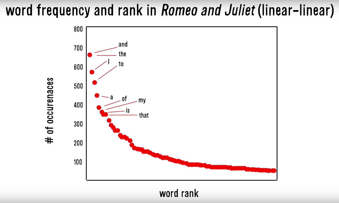
This pattern, where a few words appear very frequently while most words appear rarely, is known as Zipf’s Law. It’s a fundamental property of natural language.
We’ve discovered two problems with raw word counts:
Common words like “the” and “in” dominate the counts, but they tell us little about document content
Raw frequencies don’t tell us how unique or informative a word is across documents
Think about it: if a word appears frequently in one document but rarely in others (like “cheese” in our example), it’s probably more informative about that document’s content than a word that appears equally frequently in all documents (like “the”).
This realization leads us to two important questions:
How can we normalize word frequencies within each document to account for document length?
How can we adjust these frequencies to give more weight to words that are unique to specific documents?
TF-IDF (Term Frequency-Inverse Document Frequency) provides elegant solutions to both questions. Let’s see how it works in the next section.
The Need for Normalization#
TF-IDF (Term Frequency-Inverse Document Frequency) offers our first practical glimpse into representing words as distributed patterns rather than isolated units.
The TF-IDF score for a word \(t\) in document \(d\) combines two components:
\(\text{TF-IDF}(t,d) = \text{TF}(t,d) \times \text{IDF}(t)\)
where:
\(\text{TF}(t,d) = \dfrac{\text{count of term }t\text{ in document }d}{\text{total number of terms in document }d}\)
\(\text{IDF}(t) = \log\left(\dfrac{\text{total number of documents}}{\text{number of documents containing term }t}\right)\)
Note
Unlike one-hot encoding where each word is represented by a single position, TF-IDF represents each word through its pattern of occurrence across all documents. This distributed nature allows TF-IDF to capture semantic relationships: words that appear in similar documents will have similar patterns of TF-IDF scores.
Let’s see this distributed representation in action: First, let us consider a simple example with 5 documents about animals.
from sklearn.decomposition import PCA
import matplotlib.pyplot as plt
import numpy as np

# Sample documents about animals
documents = [
    "Cats chase mice in the garden",
    "Dogs chase cats in the park",
    "Mice eat cheese in the house",
    "Pets like dogs and cats need care",
    "Wild animals hunt in nature"
]
Second, we will split each document into words and create a vocabulary. This process is called tokenization.
tokens = []
vocab = set()
for doc in documents:
    tokens_in_doc = doc.lower().split()
    tokens.append(tokens_in_doc)
    vocab.update(tokens_in_doc)

# create a dictionary that maps each word to a unique index
word_to_idx = {word: i for i, word in enumerate(vocab)}
Third, we will count how many times each word appears in each document. We begin by creating a placeholder matrix tf_matrix to store the counts.
# Calculate term frequencies for each document
n_docs = len(documents) # number of documents
n_terms = len(vocab) # number of words

# This is a matrix of zeros
# with the number of rows equal to the number of words
# and the number of columns equal to the number of documents
tf_matrix = np.zeros((n_terms, n_docs))

print(tf_matrix)
[[0. 0. 0. 0. 0.]
 [0. 0. 0. 0. 0.]
 [0. 0. 0. 0. 0.]
 [0. 0. 0. 0. 0.]
 [0. 0. 0. 0. 0.]
 [0. 0. 0. 0. 0.]
 [0. 0. 0. 0. 0.]
 [0. 0. 0. 0. 0.]
 [0. 0. 0. 0. 0.]
 [0. 0. 0. 0. 0.]
 [0. 0. 0. 0. 0.]
 [0. 0. 0. 0. 0.]
 [0. 0. 0. 0. 0.]
 [0. 0. 0. 0. 0.]
 [0. 0. 0. 0. 0.]
 [0. 0. 0. 0. 0.]
 [0. 0. 0. 0. 0.]
 [0. 0. 0. 0. 0.]
 [0. 0. 0. 0. 0.]
 [0. 0. 0. 0. 0.]]
And then we count how many times each word appears in each document.
for doc_idx, tokens_in_doc in enumerate(tokens):
    for word in tokens_in_doc:
        term_idx = word_to_idx[word]
        tf_matrix[term_idx, doc_idx] += 1

print(tf_matrix)
[[0. 0. 1. 0. 0.]
 [1. 1. 0. 1. 0.]
 [0. 0. 0. 1. 0.]
 [1. 1. 1. 0. 1.]
 [0. 1. 0. 0. 0.]
 [0. 0. 1. 0. 0.]
 [1. 0. 0. 0. 0.]
 [0. 0. 0. 1. 0.]
 [1. 0. 1. 0. 0.]
 [0. 0. 0. 0. 1.]
 [0. 0. 1. 0. 0.]
 [0. 0. 0. 0. 1.]
 [1. 1. 0. 0. 0.]
 [0. 0. 0. 1. 0.]
 [0. 1. 0. 1. 0.]
 [0. 0. 0. 1. 0.]
 [0. 0. 0. 0. 1.]
 [0. 0. 0. 0. 1.]
 [1. 1. 1. 0. 0.]
 [0. 0. 0. 1. 0.]]
Fourth, we calculate the IDF for each word. IDF is defined as the logarithm of the inverse document frequency. Document frequency is the number of documents that contain the word. Note that, if a word appears multiple times in the same document, it should only be counted once!
# Calculate IDF for each term
# let's use tf_matrix to calculate the document frequency
doc_freq = np.zeros(n_terms)

# Go through each word
for term_idx in range(n_terms):

    # For each word, go through each document
    for doc_idx in range(n_docs):
        # If the word appears in the document, increment the document frequency
        if tf_matrix[term_idx, doc_idx] > 0:
            doc_freq[term_idx] += 1

idf = np.log(n_docs / doc_freq)
Next, we calculate the TF-IDF matrix. tf_matrix is a matrix of n_terms by n_docs, and idf is a vector of length n_terms. Remind that the tf-idf is given by
\( \text{TF-IDF}(t,d) = \text{TF}(t,d) \times \text{IDF}(t) \)
A naive way to do this (albeit not efficient) is to perform this using for loops
# Calculate TF-IDF matrix

tfidf_matrix = np.zeros((n_terms, n_docs))
for term_idx in range(n_terms):
    for doc_idx in range(n_docs):
        tfidf_matrix[term_idx, doc_idx] = tf_matrix[term_idx, doc_idx] * idf[term_idx]
A more efficient way is to use matrix multiplication.
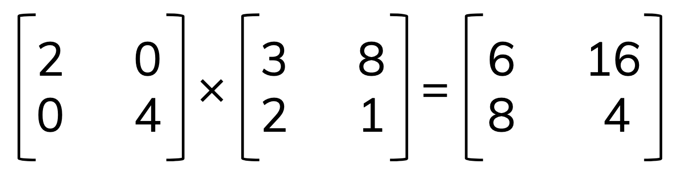
tfidf_matrix = np.diag(idf) @ tf_matrix
where np.diag(idf) creates a diagonal matrix with idf on the diagonal.
Tip
Consider a diagonal matrix as a tool to scale the rows/columns of a matrix. If we multiple a diagonal matrix from the left, we scale the rows of the matrix. If we multiple a diagonal matrix from the right, we scale the columns of the matrix.
A more efficient way is to use einsum, which is a powerful function for performing Einstein summation convention on arrays.
tfidf_matrix = np.einsum('ij,i->ij', tf_matrix, idf)
Tip
einsum provides a concise way to express complex array manipulations and can often lead to more efficient computations. Here is a concise description of how einsum works A basic introduction to NumPy’s einsum
The general form of einsum is np.einsum(subscripts, *operands), where:
subscriptsis a string specifying the subscripts for summation as comma-separated list of subscript labelsoperandsare the input arrays
In our case, 'ij,i->ij' means:
Take the first array
tf_matrixwith dimensionsi,jTake the second array
idfwith dimensioniMultiply each row
joftf_matrixby the corresponding elementiofidfOutput has same dimensions
i,jas input
Now, we have the TF-IDF matrix as follows:
print(tfidf_matrix)
[[0.         0.         1.60943791 0.         0.        ]
 [0.51082562 0.51082562 0.         0.51082562 0.        ]
 [0.         0.         0.         1.60943791 0.        ]
 [0.22314355 0.22314355 0.22314355 0.         0.22314355]
 [0.         1.60943791 0.         0.         0.        ]
 [0.         0.         1.60943791 0.         0.        ]
 [1.60943791 0.         0.         0.         0.        ]
 [0.         0.         0.         1.60943791 0.        ]
 [0.91629073 0.         0.91629073 0.         0.        ]
 [0.         0.         0.         0.         1.60943791]
 [0.         0.         1.60943791 0.         0.        ]
 [0.         0.         0.         0.         1.60943791]
 [0.91629073 0.91629073 0.         0.         0.        ]
 [0.         0.         0.         1.60943791 0.        ]
 [0.         0.91629073 0.         0.91629073 0.        ]
 [0.         0.         0.         1.60943791 0.        ]
 [0.         0.         0.         0.         1.60943791]
 [0.         0.         0.         0.         1.60943791]
 [0.51082562 0.51082562 0.51082562 0.         0.        ]
 [0.         0.         0.         1.60943791 0.        ]]
Each row of the TF-IDF matrix is our first attempt at a distributed representation of a word. Words that appear together in the same documents frequently will have similar rows.
Just like one-hot encoding, this representation can be high-dimensional, e.g., if we have 10000 documents, each word is represented by a vector of length 10000. One can reduce the dimensionality of the representation using dimensionality reduction techniques (e.g., PCA, SVD) while maintaining the structure of the data. This is possible because tf-idf matrix is often low-rank in practice.
Note
TF-IDF matrices are often low-rank because documents naturally group into clusters based on topics or themes. This clustering creates redundancy in the term-document matrix, as many terms are specific to certain clusters and rare in others. Consequently, the TF-IDF matrix can be approximated by a lower-rank matrix. This low-rank nature is useful for applications like dimensionality reduction and topic modeling, as it simplifies data visualization and analysis.
Let us apply PCA to reduce the dimensionality of the tf-idf matrix.
reducer = PCA(n_components=2)
xy = reducer.fit_transform(tfidf_matrix)
Let’s visualize the result using Bokeh.
from bokeh.plotting import figure, show, output_notebook
from bokeh.models import ColumnDataSource
from bokeh.io import push_notebook
from bokeh.plotting import figure, show
from bokeh.io import output_notebook
from bokeh.models import ColumnDataSource, HoverTool

output_notebook()

# Prepare data for Bokeh
source = ColumnDataSource(data=dict(
    x=xy[:, 0],
    y=xy[:, 1],
    text_x=xy[:, 0] + np.random.randn(n_terms) * 0.02,
    text_y=xy[:, 1] + np.random.randn(n_terms) * 0.02,
    term=list(word_to_idx.keys())
))

p = figure(title="Node Embeddings from Word2Vec", x_axis_label="X", y_axis_label="Y")

p.scatter('x', 'y', source=source, line_color="black", size = 30)

# Add labels to the points
p.text(x='text_x', y='text_y', text='term', source=source, text_font_size="10pt", text_baseline="middle", text_align="center")

show(p)
---------------------------------------------------------------------------
ModuleNotFoundError                       Traceback (most recent call last)
Cell In[13], line 1
----> 1 from bokeh.plotting import figure, show, output_notebook
      2 from bokeh.models import ColumnDataSource
      3 from bokeh.io import push_notebook

ModuleNotFoundError: No module named 'bokeh'
The power of TF-IDF lies in its ability to transform the distributional hypothesis into a practical mathematical framework. By representing words through their patterns of usage across documents, TF-IDF creates a distributed representation where semantic relationships emerge naturally from the data.
However, TF-IDF has its limitations. It only captures word-document relationships, missing out on the rich word-word relationships that occur within documents. This limitation led researchers to develop more sophisticated techniques like word2vec, which we’ll explore in the next section.