Transformers#
Transformers are the cornerstone of modern NLP that gives rise to the recent success of LLMs. We will learn how transformers work and how they are used to build LLMs.
A building block of LLMs#
Many large language models (LLMs) including GPT-3, GPT-4, and Claude are built based on a stack of transformer blocks [1]. Each transformer block takes a sequence of token vectors as input and outputs a sequence of token vectors (sequence-to-sequence!).
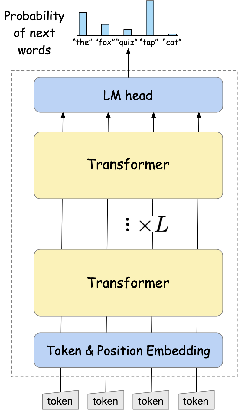
Fig. 18 The basic architecture of the transformer-based LLMs.#
These transformer blocks can be further divided into encoder and decoder components. The encoder is used for encoding the input sequence, while the decoder is used for generating the output sequence. Like seq2se models with attention, the decoder can also see the encoder outputs for invidiual tokens, along with the previous output tokens. The output of the decoder is then passed through a linear layer to produce the probability distribution over the next token.
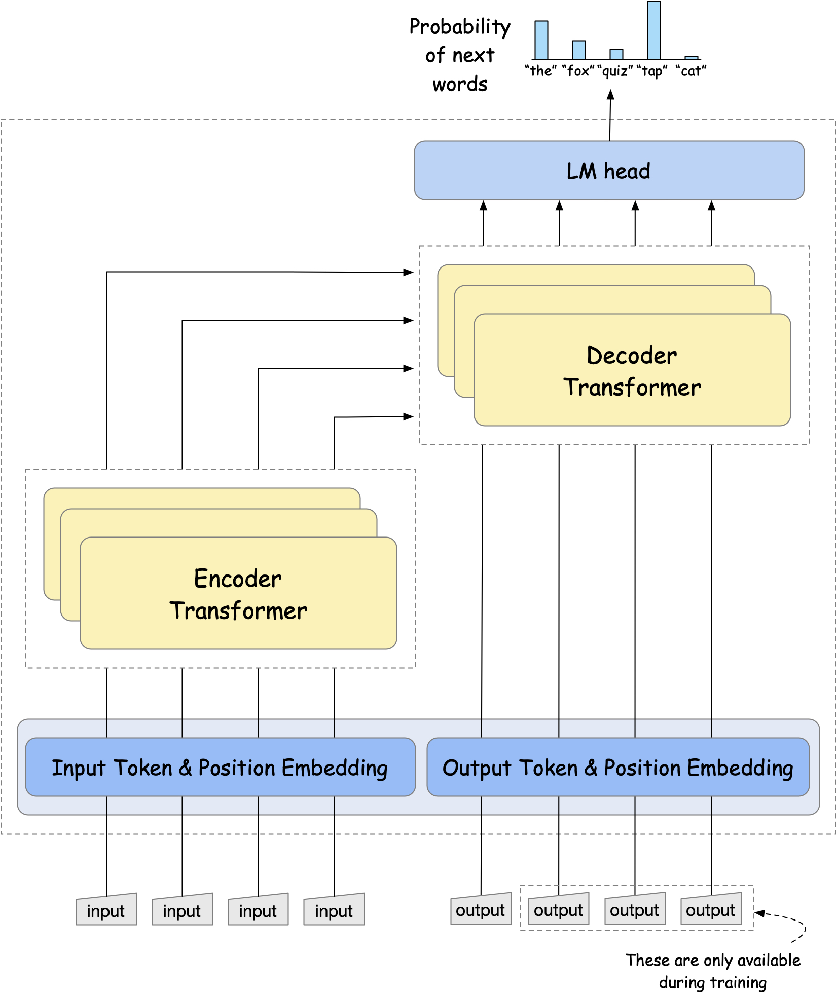
Fig. 19 The basic architecture of the transformer encoder-decoder. The encoder is used for encoding the input sequence, while the decoder is used for generating the output sequence. The encoder takes the input sequence as input and outputs a sequence of token vectors, which are then passed to the decoder. The decoder takes the encoder outputs, along with the previous output tokens, and outputs the probability distribution over the next token.#
Inside the encoder and decoder transformer blocks are essentially three components, i.e., multi-head attention, layer normalization, and feed-forward networks. We will learn individual components in the following sections.
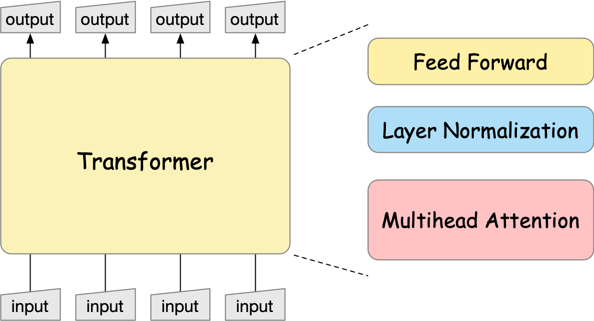
Fig. 20 The encoder-decoder architecture of the transformer.#
Attention Mechanism#
Perhaps the most crucial component of the transformer is the attention mechanism, which allows the model to pay attention to particular parts of the input sequence.
Self-Attention#
In transformers, the attention is called self-attention, since the attention is paid within the same sentence, unlike the sequence-to-sequence models that pays attention from one sentence to another. At its core, self-attention is about relationships. When you read the sentence “The cat sat on the mat because it was tired”, how do you know what “it” refers to? You naturally look back at the previous words and determine that “it” refers to “the cat”. Self-attention works similarly, but does this for every word in relation to every other word, simultaneously.
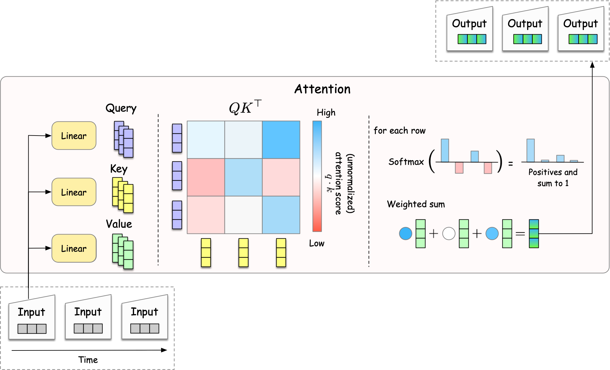
Fig. 21 The attention mechanism in transformers.#
To compute the attention between words, the attention head creates three types of vectors—query, key, and value—for each word. Each of these vectors are created by a neural network (w/ single linear layer) that takes the input word as input, and outputs another vector.
Note
Think of this like a library system: The Query is what you’re looking for, the Keys are like book titles, and the Values are the actual content of the books. When you search (Q) for a specific topic, you match it against book titles (K) to find the relevant content (V).
The query and key vectors are used to compute the attention score, which represents how much attention the model pays to each key word for the query word, with a larger score indicating a stronger attention. For example, in the sentence “The cat sat on the mat because it was tired”, a good model should pay more attention to “cat” than “mat” for the word “it”. The atttention score computed by the dot product of the query and key vectors. The score is then normalized by the softmax function, with rescaling by \(\sqrt{d_k}\) to prevent the score from becoming too large. More formally, the attention score is computed as:
where \(Q \in \mathbb{R}^{n \times d_k}\) is the query matrix containing \(n\) query vectors of dimension \(d_k\), \(K \in \mathbb{R}^{n \times d_k}\) is the key matrix containing \(n\) key vectors of dimension \(d_k\), and \(V \in \mathbb{R}^{n \times d_v}\) is the value matrix containing \(n\) value vectors of dimension \(d_v\).
The normalized attention score is used as a weight for the weghted sum of the value vectors, which results in the contextualized vector of the query word. Putting all the pieces together, the attention mechanism is computed as:
where \(V \in \mathbb{R}^{n \times d_v}\) is the value matrix containing \(n\) value vectors of dimension \(d_v\). In the original paper on transformers [1], the dimension of the query, key, and value vectors are all set to be the same, i.e., \(d_k = d_v = d_q = d / h\), where \(h\) is the number of attention heads and \(d\) is the dimension of the input vector, though this is not a strict requirement.
Note
The output of the attention mechanism is the contextualized vector, meaning that the vector for a word can vary depending on other words input to the attention module. This is ideal for language modeling, since the meaning of a word can vary depending on the context, e.g., “bank” can mean “river bank” or “financial institution” depending on the words surrounding it.
Multi-Head Attention#
Multi-head attention consists of multiple attention heads to enable a model to pay attentions to multiple aspects of the input sequence. Each attention head can have different parameters and thus produces different “contextualized vectors.” These different vector are then concatenated and fed into a feed-forward network to produce the final output.
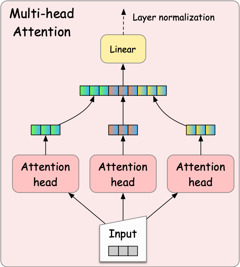
Fig. 22 Multi-head attention mechanism.#
Layer Normalization#
Fig. 23 Layer normalization works by normalizing each individual sample across its features. For each sample, it calculates the mean and standard deviation across all feature dimensions, then uses these statistics to normalize that sample’s values.#
Layer normalization is a technique used to stabilize the training of deep neural networks. It mitigates the problem of too large or too small input values, which can cause the network to become unstable. This normalization shifts and scales the input values to prevent this issue. More specifically, the layer normalization is computed as:
where \(\mu\) and \(\sigma\) are the mean and standard deviation of the input, \(\gamma\) is the scaling factor, and \(\beta\) is the shifting factor. The variables \(\gamma\) and \(\beta\) are learnable parameters that are initialized to 1 and 0, respectively, and are updated during training.
Wiring it all together#
Encoder Transformer Block#
Now, we have all the components to build a transformer block. Let’s wire them together.
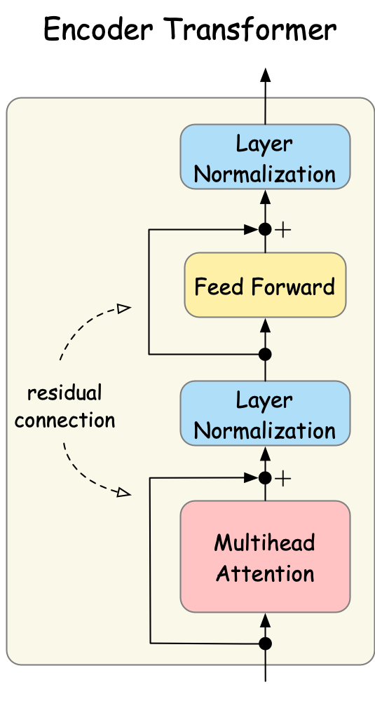
Fig. 24 Input flows through multi-head attention, layer normalization, feed-forward networks, and another normalization step.#
Let us ignore the residual connection for now. The input is first passed through multi-head attention, followed by layer normalization. Then, the output of the normalization is passed through feed-forward networks and another layer normalization step.
Residual Connection#
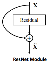
Fig. 25 Residual connection.#
Now, let us consider the residual connection. A residual connection, also known as a skip connection, is a technique used to stabilize the training of deep neural networks. More specifically, let us denote by \(f\) the neural network that we want to train, which is the multi-head attention or feed-forward networks in the transformer block. The residual connection is defined as:
Note that rather than learning the complete mapping from input to output, the network \(f\) learns to model the residual (difference) between them. This is particularly advantageous when the desired transformation approximates an identity mapping, as the network can simply learn to output values near zero.
Residual connections help prevent the vanishing gradient problem. Deep learning models like LLMs consist of many layers, which are trained to minimize the loss function \({\cal L}_{\text{loss}}\) with respect to the parameters \(\theta\). To this end, the gradient of the loss function is computed using the chain rule as
where \(f_i\) is the output of the \(i\)-th layer. The gradient vanishing problem occurs when the individual terms \(\frac{\partial f_{i+1}}{\partial f_i}\) are less than 1. As a result, the gradient becomes smaller and smaller as the gradient flows backward through earlier layers. By adding the residual connection, the gradient for the individual term becomes:
Notice the “+1” term, which is the direct path from the input to the output. The chain rule is thus modified as:
When we expand this, we can group terms by their order (how many \(\partial f_i\) terms are multiplied together): We can write this more concisely using \(O_n\) to represent terms of nth order:
where:
\(O_1 = \frac{\partial f_{L-1}}{\partial x_{L-1}} + \frac{\partial f_{L-2}}{\partial x_{L-2}} + \frac{\partial f_{L-3}}{\partial x_{L-3}} + ...\)
\(O_2 = \frac{\partial f_{L-1}}{\partial x_{L-1}}\frac{\partial f_{L-2}}{\partial x_{L-2}} + \frac{\partial f_{L-2}}{\partial x_{L-2}}\frac{\partial f_{L-3}}{\partial x_{L-3}} + \frac{\partial f_{L-1}}{\partial x_{L-1}}\frac{\partial f_{L-3}}{\partial x_{L-3}} + ...\)
\(O_3 = \frac{\partial f_{L-1}}{\partial x_{L-1}}\frac{\partial f_{L-2}}{\partial x_{L-2}}\frac{\partial f_{L-3}}{\partial x_{L-3}} + ...\)
Without the residual connection, we only have the \(O_L\) terms for the network with \(L\) layers, which is subject to the gradient vanishing problem. Whereas with the residual connection, we have the lower-order terms like \(O_1, O_2, O_3, ...\) for the network with \(L\) layers, which is less susceptible to the gradient vanishing problem.
Residual Connection
Residual connections are a architectural innovation that allows neural networks to be much deeper without degrading performance. It was proposed by He et al. for image processing from Microsoft Research.
Residual connection mitigates gradient explosion
Residual connections also help prevent gradient explosion, even though this may not be obvious from the chain rule perspective. As shown in [2], the residual connection provides an alternative path for gradients to flow through. By distributing gradients between the residual path and the learning component path, the gradient is less likely to explode.
Decoder Transformer Block#
The decoder transformer block is similar to the encoder transformer block, but it also includes the masked multi-head attention and cross-attention components.
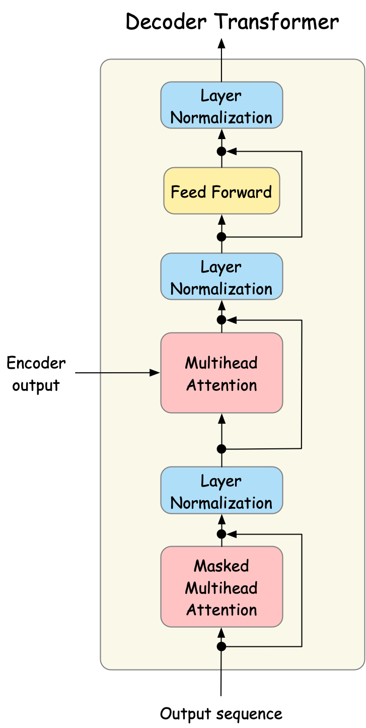
Fig. 26 The decoder transformer block.#
Masked Multi-Head Attention#
The masked multi-head attention is used during training to prevent the decoder from seeing the future tokens. During inference, the masked mult-head attention acts as a regular attention module.
The masked multi-head attention is crucial for enabling parallel training of the decoder. During training, we know the entire expected output sequence, but we need to ensure the model learns to generate tokens sequentially without “peeking” at future tokens.
Let’s understand this with an example. Suppose we’re training a model to translate “I love you” to French “Je t’aime”. The encoder processes the input sequence in parallel, producing vector representations (say 11, 12, 13 for simplicity). For the decoder training, we have two options:
Sequential Training (without masking): Process one token at a time
Step 1: Input (11,12,13) → Predict “Je”
Step 2: Input (11,12,13) + predicted “Je” → Predict “t’aime”
Step 3: Input (11,12,13) + predicted “t’aime” → Predict final token
This is slow and errors accumulate across steps.
Parallel Training (with masking): Process all tokens simultaneously
Operation A: Input (11,12,13) → Predict “Je” (mask out “t’aime”)
Operation B: Input (11,12,13) + “Je” → Predict “t’aime” (mask out final token)
Operation C: Input (11,12,13) + “Je” + “t’aime” → Predict final token
The parallel training is much faster and more efficient, since the model can process all tokens simultaneously. Additionally, the model does not suffer from the error accumulation problem, where the prediction error from one step is carried over to the next step.
To implement the masking, we set the attention scores to negative infinity for future tokens before the softmax operation, effectively zeroing out their contribution:
where \(M\) is a matrix with \(-\infty\) for positions corresponding to future tokens. The result is the attention scores, where the tokens attend only to the previous tokens.
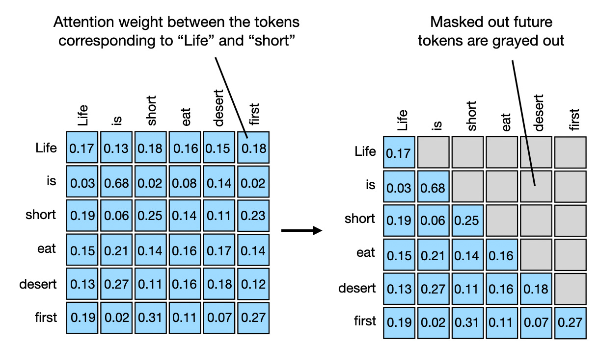
Fig. 27 The masked attention mechanism.#
Cross-Attention#
Cross-attention is the second multi-head attention component in the decoder transformer block. It creates a connection between the decoder and encoder by allowing the decoder to access information from the encoder’s output.
The mechanism works by using queries (Q) from the decoder’s previous layer and keys (K) and values (V) from the encoder’s output. This enables each position in the decoder to attend to the full encoder sequence without any masking, since encoding is already complete.
For instance, in translating “I love you” to “Je t’aime”, cross-attention helps each French word focus on relevant English words - “Je” attending to “I”, and “t’aime” to “love”. This maintains semantic relationships between input and output.
The cross-attention formula is:
where Q comes from the decoder and K,V come from the encoder. This effectively bridges the encoding and decoding processes.
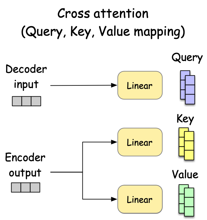
Fig. 28 The cross-attention mechanism.#
Other miscellaneous components#
Position embedding#
Position embedding is also an interesting component that is used to encode the position of the tokens in the sequence. A key limitation of the attention mechanism is that it is permutation invariant. This means that the order of the input tokens does not matter, e.g., “The cat sat on the mat” and “The mat sat on the cat” are the same. To better capture the position information, transformers add to the input token embedding a position embedding.
To understand how this works, let us approach from a naive approach. Suppose that we have a sequence of \(T\) token embeddings, denoted by \(x_1, x_2, ..., x_T\), each of which is a \(d\)-dimensional vector. A simple way to encode the position information is to add a position index to each token embedding, i.e.,
where \(t = 1, 2, ..., T\) is the position index of the token in the sequence, and \(\beta\) is the step size. This appears to be simple but has a critical problem.
Unbounded: The position index can be arbitrarily large. When the models see a sequence longer than those in training data, it may suffer since the model will be exposed to a new position index that the model has never seen before.
Discrete: The position index is discrete, which means that the model cannot capture the position information in a smooth manner.
Because this naive approach has the problems, let us consider another approach. Let us represent the position index using a binary vector of length \(d\). For example, in case of \(d=4\), we have the following binary vectors:
Then, one may use the binary vector as the position embedding as follows:
where \(\text{Pos}(t, i)\) is the position embedding vector of the position index \(t\) and the dimension index \(i\). This representation is good in the sense that it is unbounded. Yet, it is still discrete.
An elegant position embedding, which is used in transformers, is the sinusoidal position embedding [1]. It appears to be complicated but stay with me for a moment.
where \(i\) is the dimension index of the position embedding vector. This position embedding is added to the input token embedding as:
It appears to be complicated but it can be seen as a continuous version of the binary position embedding above. To see this, let us plot the position embedding for the first 100 positions.
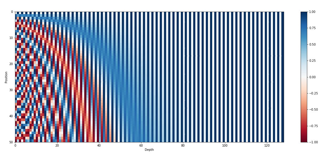
Fig. 29 The position embedding. The image is taken from https://kazemnejad.com/blog/transformer_architecture_positional_encoding/#
We note that, just like the binary position embedding, the sinusoidal position embedding also exhibits the alternating pattern (vertically) with frequency increasing as the dimension index increases (horizontal axis). Additionally, the sinusoidal position embedding is continuous, which means that the model can capture the position information in a smooth manner.
Another key property of the sinusoidal position embedding is that the dot similarity between the two position embedding vectors represent the similarity between the two positions, regardless of the position index.
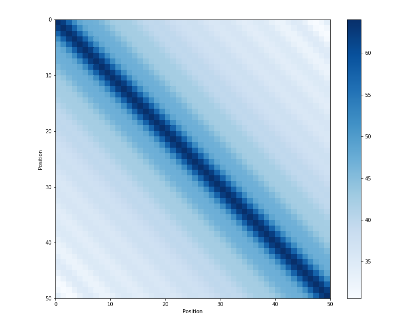
Fig. 30 :name: transformer-position-embedding-similarity :alt: Transformer Position Embedding Similarity :width: 80% :align: center#
The dot similarity between the two position embedding vectors represent the distance between the two positions, regardless of the position index. The image is taken from https://kazemnejad.com/blog/transformer_architecture_positional_encoding/
Why additive position embedding?
The sinusoidal position embedding is additive, which alter the token embedding. Alternatively, one may concatenate, instead of adding, the position embedding to the token embedding, i.e., \(x_{t,i} := [x_{t,i}; \text{Pos}(t, i)]\). This makes it easier for a model to distinguish the position information from the token information. So why not use the concatenation?
One reason is that the concatenation requires a larger embedding dimension, which increases the number of parameters in the model. Instead, adding the position embedding creates an interesting effect in the attention mechanism. Interested readers can check out this Reddit post.
Absolute vs Relative Position Embedding
Absolute position embedding is the one we discussed above, where each position is represented by a unique vector. On the other hand, relative position embedding represents the position difference between two positions, rather than the absolute position [3]. The relative position embedding can be implemented by adding a learnable scalar to the unnormalized attention scores before softmax operation [4], i.e.,
where \(B\) is a learnable offset matrix that is added to the unnormalized attention scores. The matrix \(B\) is a function of the position difference between the query and key, i.e., \(B = f(i-j)\), where \(i\) and \(j\) are the position indices of the query and key, respectively. Such a formulation is useful when the model needs to capture the relative position between two tokens.