Bidirectional Encoder Representations from Transformers (BERT)#
We learned about ELMo’s approach to the problem of polysemy using bidirectional LSTMs. BERT builds upon its bidirectional approach by using a self-attention mechanism in transformers. BERT has become the leading transformer model for natural language processing tasks like question answering and text classification. Its effectiveness led Google to incorporate it into their search engine to improve query understanding. In this section, we will explore BERT’s architecture and mechanisms.
BERT in interactive mode:
Here is a demo notebook for BERT
To run the notebook, download the notebook as a .py file and run it with:
marimo edit –sandbox bert.py
You will need to install marimo and uv to run the notebook. But other packages will be installed automatically in uv’s virtual environment.
Architecture#
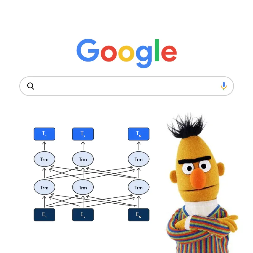
BERT consists of a stack of encoder transformer layers. Each layer is composed of a self-attention mechanism, a feed-forward neural network, and layer normalization, wired together with residual connections. The output of each layer is fed into the next layer, and as we go through the layers, the token embeddings get more and more contextualized, reflecting the context more and more, thanks to the self-attention mechanism.
Fig. 31 BERT consists of a stack of encoder transformer layers. The position embeddings are added to the token embeddings to provide the model with information about the position of the tokens in the sequence.#
Which layer of BERT should we use?
BERT internally generates multiple hierarchical representations of the input sentence. The higher layers of the model capture more abstract and context-sensitive information, while the lower layers capture more local and surface-level information. Which layer to use depends on the task. For example, if we want to do text classification, we should use the output of the last layer. If we are interested in word-level representations, we should use the output of the first layer.
Special tokens#
BERT uses several special tokens to represent the input sentence.
[CLS] is used to represent the start of the sentence.
[SEP] is used to represent the end of the sentence.
[MASK] is used to represent the masked words.
[UNK] is used to represent the unknown words.
For example, the sentence “The cat sat on the mat. It then went to sleep.” is represented as “[CLS] The cat sat on the mat [SEP] It then went to sleep [SEP]”.
In BERT, [CLS] token is used to classify the input sentences, as we will see later. As a result, the model learns to encode a summary of the input sentence into the [CLS] token, which is particularly useful when we want the embedding of the whole input text, instead of the token level embeddings. [1]
Position and Segment embeddings#
BERT uses position and segment embeddings to provide the model with information about the position of the tokens in the sequence.
Position embeddings are used to provide the model with information about the position of the tokens in the sequence. Unlike the sinusoidal position embedding used in the original transformer paper [2], BERT uses learnable position embeddings.
The segment embeddings are used to distinguish the sentences in the input. For example, for the sentence “The cat sat on the mat. It then went to sleep.”, the tokens in the first sentence are added with segment embedding 0, and the tokens in the second sentence are added with segment embedding 1. These segmend embeddings are also learned during the pre-training process.

Fig. 32 Position and segment embeddings in BERT. Position embeddings, which are learnable, are added to the token embeddings. Segment embeddings indicate the sentence that the token belongs to (e.g., \(E_A\) and \(E_B\)).#
Tip
Position embeddings can be either absolute or relative:
Absolute position embeddings (like in BERT) directly encode the position of each token as a fixed index (1st, 2nd, 3rd position etc). Each position gets its own unique embedding vector that is learned during training.
Relative position embeddings (like sinusoidal embeddings in the original Transformer) encode the relative distance between tokens rather than their absolute positions. For example, they can encode that token A is 2 positions away from token B, regardless of their absolute positions in the sequence. This makes them more flexible for handling sequences of varying lengths.
For interested readers, you can read more about the difference between absolute and relative position embeddings in The Use Case for Relative Position Embeddings – Ofir Press and Train Short, Test Long: Attention with Linear Biases Enables Input Length Extrapolation.
Pre-training#
A key aspect of BERT is its pre-training process, which involves two main objectives:
Masked Language Modeling (MLM)
Next Sentence Prediction (NSP)
Both objectives are designed to learn the language structure, such as the relationship between words and sentences.
Masked Language Modeling (MLM)#
In MLM, the model is trained to predict the original words that are masked in the input sentence. The masked words are replaced with a special token, [MASK], and the model is trained to predict the original words. For example, the sentence “The cat [MASK] on the mat” is transformed into “The cat [MASK] on the mat”. The model is trained to predict the original word “sat” in the sentence.
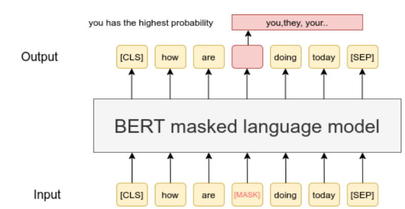
Fig. 33 Masked Language Modeling (MLM). A token is randomly masked and the model is trained to predict the original word.#
To generate training data for MLM, BERT randomly masks 15% of the tokens in each sequence. However, the masking process is not as straightforward as simply replacing words with [MASK] tokens. For the 15% of tokens chosen for masking:
80% of the time, replace the word with the [MASK] token
Example: “the cat sat on the mat” → “the cat [MASK] on the mat”
10% of the time, replace the word with a random word
Example: “the cat sat on the mat” → “the cat dog on the mat”
10% of the time, keep the word unchanged
Example: “the cat sat on the mat” → “the cat sat on the mat”
The model must predict the original token for all selected positions, regardless of whether they were masked, replaced, or left unchanged. This helps prevent the model from simply learning to detect replaced tokens.
During training, the model processes the modified input sequence through its transformer layers and predicts the original token at each masked position using the contextual representations.
Tip
While replacing words with random tokens or leaving them unchanged may seem counterintuitive, research has shown this approach is effective [3]. It has become an essential component of BERT’s pre-training process.
Next Sentence Prediction (NSP)#
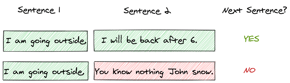
Fig. 34 Next Sentence Prediction (NSP). The model is trained to predict whether two sentences are consecutive or not.#
Next Sentence Prediction (NSP) trains BERT to understand relationships between sentences. The model learns to predict whether two sentences naturally follow each other in text. During training, half of the sentence pairs are consecutive sentences from documents (labeled as IsNext), while the other half are random sentence pairs (labeled as NotNext).
The input format uses special tokens to structure the sentence pairs: a [CLS] token at the start, the first sentence, a [SEP] token, the second sentence, and a final [SEP] token. For instance:
BERT uses the final hidden state of the [CLS] token to classify whether the sentences are consecutive or not. This helps the model develop a broader understanding of language context and relationships between sentences.
These two objectives help BERT learn the structure of language, such as the relationship between words and sentences.
Fine-tuning#
A powerful aspect of BERT is its ability to be fine-tuned on a wide range of tasks with minimal changes to the model architecture. This is achieved through transfer learning, where the pre-trained BERT model is used as a starting point for specific tasks.
Consider a hospital that wants to classify patient reviews. Due to privacy concerns, collecting enough data to train a deep learning model from scratch would be difficult. This is where BERT shines - since it’s already pre-trained on vast amounts of text data and understands language structure, it can be fine-tuned effectively even with a small dataset of patient reviews. The pre-trained BERT model can be adapted to this specific classification task with only minor architectural changes.
Tip
You can find many fine-tuned and pre-trained models for various tasks by searching the Hugging Face model hub, with the keyword “BERT”.
Variants and improvements#
RoBERTa (Robustly Optimized BERT Approach) [4] improved upon BERT through several optimizations: removing the Next Sentence Prediction task, using dynamic masking that changes the mask patterns across training epochs, training with larger batches, and using a larger dataset. These changes led to significant performance improvements while maintaining BERT’s core architecture.
DistilBERT [5] focused on making BERT more efficient through knowledge distillation, where a smaller student model learns from the larger BERT teacher model. It achieves 95% of BERT’s performance while being 40% smaller and 60% faster, making it more suitable for resource-constrained environments and real-world applications.
ALBERT [6] introduced parameter reduction techniques to address BERT’s memory limitations. It uses factorized embedding parameterization and cross-layer parameter sharing to dramatically reduce parameters while maintaining performance. ALBERT also replaced Next Sentence Prediction with Sentence Order Prediction, where the model must determine if two consecutive sentences are in the correct order.
Domain-specific BERT models have been trained on specialized corpora to better handle specific fields. Examples include BioBERT [7] for biomedical text, SciBERT [1] for scientific papers, and FinBERT [8] for financial documents. These models demonstrate superior performance in their respective domains compared to the general-purpose BERT.
Multilingual BERT (mBERT) [4] was trained on Wikipedia data from 104 languages, using a shared vocabulary across all languages. Despite not having explicit cross-lingual objectives during training, mBERT shows remarkable zero-shot cross-lingual transfer abilities, allowing it to perform tasks in languages it wasn’t explicitly aligned on. This has made it a valuable resource for low-resource languages and cross-lingual applications.
Hands on#
Let us load a pre-trained BERT model and see how it works using a sense disambiguation task. The sense disambiguation task is a task that involves identifying the correct sense of a word in a sentence. For example, given a sentence with word “apple”, we need to identify whether it refers to the fruit or the technology company.
Let us first load the necessary libraries.
import pandas as pd
import numpy as np
import sys
import torch
import transformers
import matplotlib.pyplot as plt
from tqdm import tqdm
from sklearn.decomposition import PCA
from bokeh.plotting import figure, show
from bokeh.io import output_notebook
from bokeh.models import ColumnDataSource, HoverTool
---------------------------------------------------------------------------
ImportError                               Traceback (most recent call last)
Cell In[1], line 4
      2 import numpy as np
      3 import sys
----> 4 import torch
      5 import transformers
      6 import matplotlib.pyplot as plt

File ~/miniforge3/envs/applsoftcomp/lib/python3.10/site-packages/torch/__init__.py:367
    365     if USE_GLOBAL_DEPS:
    366         _load_global_deps()
--> 367     from torch._C import *  # noqa: F403
    370 class SymInt:
    371     """
    372     Like an int (including magic methods), but redirects all operations on the
    373     wrapped node. This is used in particular to symbolically record operations
    374     in the symbolic shape workflow.
    375     """

ImportError: dlopen(/Users/skojaku-admin/miniforge3/envs/applsoftcomp/lib/python3.10/site-packages/torch/_C.cpython-310-darwin.so, 0x0002): Symbol not found: __ZN2at3cpu20is_arm_sve_supportedEv
  Referenced from: <D93D20A5-7F4C-32F1-874B-FE7B416FFD91> /Users/skojaku-admin/miniforge3/envs/applsoftcomp/lib/python3.10/site-packages/torch/lib/libtorch_python.dylib
  Expected in:     <616791F0-29C3-3F88-8A88-D072E7E40979> /Users/skojaku-admin/miniforge3/envs/applsoftcomp/lib/libtorch_cpu.dylib
We will use CoarseWSD-20. The dataset contains sentences with polysemous words and their sense labels. We will see how to use BERT to disambiguate the word senses. Read the README for more details.
def load_data(focal_word, is_train, n_samples=100):
    data_type = "train" if is_train else "test"
    data_file = f"https://raw.githubusercontent.com/danlou/bert-disambiguation/master/data/CoarseWSD-20/{focal_word}/{data_type}.data.txt"
    label_file = f"https://raw.githubusercontent.com/danlou/bert-disambiguation/master/data/CoarseWSD-20/{focal_word}/{data_type}.gold.txt"

    data_table = pd.read_csv(
        data_file,
        sep="\t",
        header=None,
        dtype={"word_pos": int, "sentence": str},
        names=["word_pos", "sentence"],
    )
    label_table = pd.read_csv(
        label_file,
        sep="\t",
        header=None,
        dtype={"label": int},
        names=["label"],
    )
    combined_table = pd.concat([data_table, label_table], axis=1)
    return combined_table.sample(n_samples)


focal_word = "apple"

train_data = load_data(focal_word, is_train=True)

train_data.head(10)
We will use transformers library developed by Hugging Face to define the BERT model. To use the model, we will need:
BERT tokenizer that converts the text into tokens.
BERT model that computes the embeddings of the tokens.
We will use the bert-base-uncased model and tokenizer. Let’s define the model and tokenizer.
tokenizer = transformers.AutoTokenizer.from_pretrained("bert-base-uncased")
model = transformers.AutoModel.from_pretrained("bert-base-uncased")
model.eval() # set the model to evaluation mode
print(model) # Print the model architecture
This prints the model architecture, which shows:
BertEmbeddings layer that converts tokens into embeddings using:
Word embeddings (30522 vocab size, 768 dimensions)
Position embeddings (512 positions, 768 dimensions)
Token type embeddings (2 types, 768 dimensions)
Layer normalization and dropout
BertEncoder with 12 identical BertLayers, each containing:
Self-attention mechanism with query/key/value projections
Intermediate layer with GELU activation
Output layer with layer normalization
BertPooler that processes the [CLS] token embedding with:
Dense layer (768 dimensions)
Tanh activation
All layers maintain the 768-dimensional hidden size, except the intermediate layer which expands to 3072 dimensions.
With BERT, we need to prepare text in ways that BERT can understand. Specifically, we prepend it with [CLS] and append [SEP]. We will then convert the text to a tensor of token ids, which is ready to be fed into the model.
def prepare_text(text):
    text = "[CLS] " + text + " [SEP]"
    tokenized_text = tokenizer.tokenize(text)
    indexed_tokens = tokenizer.convert_tokens_to_ids(tokenized_text)

    segments_ids = torch.ones((1, len(indexed_tokens)), dtype=torch.long)
    tokens_tensor = torch.tensor([indexed_tokens])
    segments_tensor = segments_ids.clone()
    return tokenized_text, tokens_tensor, segments_tensor
Let’s get the BERT embeddings for the sentence “Bank is located in the city of London”.
text = "Bank is located in the city of London"
tokenized_text, tokens_tensor, segments_tensor = prepare_text(text)
This produces the following output. Tokenized text:
print(tokenized_text)
Token IDs:
print(tokens_tensor)
Segment IDs:
print(segments_tensor)
Then, let’s get the BERT embeddings for each token.
# Configure model to return hidden states
model.config.output_hidden_states = True

outputs = model(tokens_tensor, segments_tensor)
The output includes loss, logits, and hidden_states. We will use hidden_states, which contains the embeddings of the tokens.
hidden_states = outputs.hidden_states

print("how many layers? ", len(hidden_states))
print("Shape? ", hidden_states[0].shape)
The hidden states are a list of 13 tensors, where each tensor is of shape (batch_size, sequence_length, hidden_size). The first tensor is the input embeddings, and the subsequent tensors are the hidden states of the BERT layers.
So, we have 13 choice of hidden states. Deep layers close to the output capture the context of the word from the previous layers.
Here we will take the average over the last four hidden states for each token.
last_four_layers = hidden_states[-4:]
# Stack the layers and then calculate mean
stacked_layers = torch.stack(last_four_layers)
emb = torch.mean(stacked_layers, dim=0)

print(emb.shape)
emb is of shape (sequence_length, hidden_size). Let us summarize the embeddings of the tokens into a function.
def get_bert_embeddings(text):
    tokenized_text, tokens_tensor, segments_tensor = prepare_text(text)
    outputs = model(tokens_tensor, segments_tensor)
    hidden_states = outputs[2]  # Access hidden states from tuple output
    # Stack the last 4 layers then take mean
    stacked_layers = torch.stack(hidden_states[-4:])
    emb = torch.mean(stacked_layers, dim=0)
    return emb, tokenized_text
Now, let us embed text and get the embeddings of the focal token.
labels = []  # label
emb = []  # embedding
sentences = []  # sentence

def get_focal_token_embedding(text, focal_word_idx):
    emb, tokenized_text = get_bert_embeddings(text)
    return emb[0][focal_word_idx]  # Access first batch dimension

for index, row in train_data.iterrows():
    text = row["sentence"]
    focal_word_idx = row["word_pos"]
    _emb = get_focal_token_embedding(text, focal_word_idx)
    labels.append(row["label"])
    emb.append(_emb)
    sentences.append(text)
Finally, let us visualize the embeddings using PCA.
Show code cell source
# Convert list of tensors to numpy array
emb_numpy = torch.stack(emb).detach().numpy()

pca = PCA(n_components=2, random_state=42)
xy = pca.fit_transform(emb_numpy)

output_notebook()

# Create data source for Bokeh
source = ColumnDataSource(data=dict(
    x=xy[:, 0],
    y=xy[:, 1],
    label=labels,
    sentence=sentences
))

# Create Bokeh figure
p = figure(title="Word Embeddings Visualization", x_axis_label="PCA 1", y_axis_label="PCA 2",
           width=700, height=500)

# Add hover tool
hover = HoverTool(tooltips=[
    ('Label', '@label'),
    ('Sentence', '@sentence')
])
p.add_tools(hover)

# Create color map for labels
import seaborn as sns

unique_labels = list(set(labels))
color_map = sns.color_palette().as_hex()[0:len(unique_labels)]
source.data['color'] = [color_map[label] for label in labels]

# Add scatter plot
p.scatter('x', 'y', size=12, line_color="DarkSlateGrey", line_width=2,
         fill_color='color', source=source)

show(p)
Exercise#
We have used the last 4 layers of BERT to generate the embeddings of the tokens. Now, let’s use the last \(k = 1, 2, 3\) layers of BERT to generate the embeddings of the tokens. Then plot the embeddings using PCA.