GoogleNet and the Inception Module

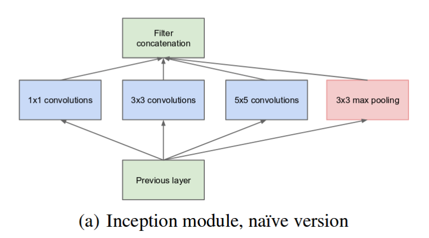
Imagine you’re looking at a painting in an art gallery. You might step close to examine the tiny brushstrokes or stand far away to observe the overall composition. How can a neural network do something similar with images? The Inception module proposed by Szegedy et al. in “Going Deeper with Convolutions” tackles this by letting different convolutional filters (big and small) work together in parallel—capturing both fine details and large-scale context at once.

Conceptual Foundation

Multi-Scale Feature Extraction

In a traditional CNN layer, you pick one filter size (like \(3 \times 3\)). But an Inception module uses multiple filter sizes (like \(1 \times 1\), \(3 \times 3\), and \(5 \times 5\)) all at once. Each filter “looks” at the same input but focuses on different scales—much like zooming in and out of a scene.

Sparse Connectivity by 1x1 Convolutions

From a theoretical perspective, not every pixel in a feature map needs to connect to every pixel in the next layer (i.e., connectivity is often sparse). However, sparse operations can be slow on current hardware. Inception approximates this “sparse” idea by using 1x1 convolutions.

The 1x1 convolutions appear unnatural at first glance but they are actually a very elegant solution to “sparcify” the convolutional filters. The core idea is that pixel values at different spatial locations are often less correlated than the values across different channels. Thus, 1x1 convolutions focus on compressing or expanding information across channels, reducing the effective parameter count for the subsequent larger filters.

For example, for a \(3 \times 3\) convolution filter, the 1x1 convolution reduces the number of parameters from \(3 \times 3 \times C_{\text{in}} \times C_{\text{out}}\) to \(1 \times 1 \times C_{\text{in}}\) (1x1 convolution) plus \(3 \times 3 \times C_{\text{out}}\) (3x3 convolution). This is \(C_{\text{in}} + 9C_{\text{out}}\) versus \(9C_{\text{in}} \times C_{\text{out}}\), yielding a substantial parameter reduction when \(C_{\text{out}}\) or \(C_{\text{in}}\) is large.

Note

Connection to Sparse Representations Early theoretical work suggested that a sparse network with many filter sizes could approximate a wide variety of feature types. However, directly implementing a sparse network can be very memory-intensive. The Inception module cleverly approximates a sparse structure by mixing 1x1, 3x3, and 5x5 convolutions in an efficient manner.

Filter Concatenation

After each branch applies its own sequence of convolutions (or pooling), the results are merged by concatenating them along the channel dimension. Think of it as stacking the feature maps from each branch side by side. This “merge” step is powerful because:

• It combines multi-scale features into a single tensor.

• Each branch contributes a unique perspective (e.g., the \(1\times1\) branch might capture fine details, while the \(5\times5\) branch looks at broader context).

• The network can learn how to best blend and leverage these feature maps for the next stage of processing.

As a result, the final output of an Inception module is a multi-channel representation that integrates information from multiple scales and pooling operations.

Parallel Pooling

GoogleNet is a stack of the Inception modules explained above, followed by a module that transform the feature maps of the last Inception module into a single vector that is used for classification. This last module is also one of the key feature of GoogleNet that sets it apart from the previous architectures.

GoogleNet uses max pooling for each channel of the feature maps. For example, if the feature maps has 10 channel, the max pooling will reduce it to 10-dimensional vector, regardless of the spatial dimension of the feature maps, by taking the maximum value across the spatial dimension.

This design choice was motivated, in part, by observations like in VGG16 (which uses the full-connected layers to this transformation), where 123 million of its 138 million parameters come from fully-connected layers alone. Reducing or eliminating these layers via pooling can dramatically cut down on model size and overfitting risk[1].

Auxiliary Classifiers

As GoogleNet grew deeper, the authors noticed that early layers sometimes struggled with vanishing gradients. To combat this, auxiliary classifiers were placed at intermediate layers. The authors take the output from the classifier attached to these intermediate layers, and add its loss to the overall loss. When backpropagating, the gradient from the auxiliary classifier is also added to the gradient of the earlier layers, which guides the earlier layers to learn more discriminative features.

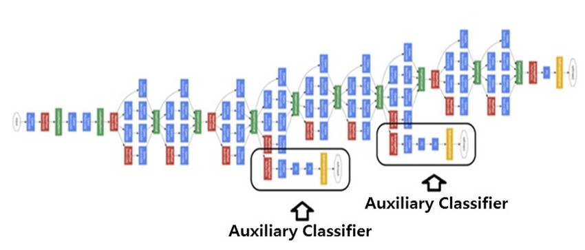
Fig. 67 An illustration of the GoogleNet architecture, including the auxiliary classifier units.

Mathematical Framework (Light Overview)

Let’s denote the input to an Inception module as a 3D tensor \( X \) with shape \((H \times W \times C)\), where \(H\) and \(W\) are the spatial dimensions and \(C\) is the channel depth.

1. 1x1 path:

   \[ Y_{1\times1} = \text{Conv}_{1\times1}(X) \]

2. 1x1 -> 3x3 path:

   \[ X_{\text{reduced}} = \text{Conv}_{1\times1}(X), \quad Y_{3\times3} = \text{Conv}_{3\times3}(X_{\text{reduced}}) \]

3. 1x1 -> 5x5 path:

   \[ X_{\text{reduced}}' = \text{Conv}_{1\times1}(X), \quad Y_{5\times5} = \text{Conv}_{5\times5}(X_{\text{reduced}}') \]

4. Pooling path:

   \[ Y_{\text{pool}} = \text{Pool}(X) \quad\text{(often followed by Conv}_{1\times1}) \]

After computing these branches, the final output of the Inception module is:

\[ Y_{\text{inception}} = \text{Concat}\big(Y_{1\times1}, \,Y_{3\times3}, \,Y_{5\times5}, \,Y_{\text{pool}}\big). \]

Recent Advancements and Improvements

1. Inception v2 & v3

   • Introduced Batch Normalization, reducing internal covariate shift.

   • Factorized larger filters (e.g., 5x5 → two 3x3) to cut cost. These improvements increased accuracy and efficiency.

2. Inception v4 & Inception-ResNet

   • Integrated residual connections, further improving training stability and depth.

3. Xception

   • Proposed depthwise separable convolutions, pushing the Inception idea further by decoupling spatial and channel-wise processing, leading to better efficiency.

4. Simplified Inception with Hadamard Attention

   • Targeted at medical image classification.

   • Uses attention mechanisms to focus on crucial parts of the image, enhancing accuracy without exploding parameter size[2].

Implementation Example

Below is a simplified PyTorch-like example of how we can define a single Inception module. This code demonstrates the parallel branches and concatenation of outputs. While not an exact reproduction of GoogleNet, it captures the core idea.

import torch
import torch.nn as nn
import torch.nn.functional as F

class InceptionModule(nn.Module):
    def __init__(self, in_channels, out_1x1, red_3x3, out_3x3, red_5x5, out_5x5, pool_proj):
        super(InceptionModule, self).__init__()

        # Branch 1: 1x1 Conv
        self.branch1 = nn.Conv2d(in_channels, out_1x1, kernel_size=1)

        # Branch 2: 1x1 Conv -> 3x3 Conv
        self.branch2_reduce = nn.Conv2d(in_channels, red_3x3, kernel_size=1)
        self.branch2 = nn.Conv2d(red_3x3, out_3x3, kernel_size=3, padding=1)

        # Branch 3: 1x1 Conv -> 5x5 Conv
        self.branch3_reduce = nn.Conv2d(in_channels, red_5x5, kernel_size=1)
        self.branch3 = nn.Conv2d(red_5x5, out_5x5, kernel_size=5, padding=2)

        # Branch 4: Max Pool -> 1x1 Conv
        self.branch4_pool = nn.MaxPool2d(kernel_size=3, stride=1, padding=1)
        self.branch4 = nn.Conv2d(in_channels, pool_proj, kernel_size=1)

    def forward(self, x):
        branch1_out = F.relu(self.branch1(x))

        branch2_out = F.relu(self.branch2(F.relu(self.branch2_reduce(x))))

        branch3_out = F.relu(self.branch3(F.relu(self.branch3_reduce(x))))

        branch4_out = F.relu(self.branch4(self.branch4_pool(x)))

        # Concatenate along channel dimension
        return torch.cat([branch1_out, branch2_out, branch3_out, branch4_out], dim=1)

# Example usage:
if __name__ == "__main__":
    inception = InceptionModule(64, 16, 16, 24, 16, 24, 16)
    dummy_input = torch.randn(1, 64, 56, 56)  # (batch_size, channels, height, width)
    output = inception(dummy_input)
    print("Output shape from Inception module:", output.shape)

Output shape from Inception module: torch.Size([1, 80, 56, 56])

Coding Exercise: Using Pre-trained GoogLeNet in PyTorch

Below is a simple exercise that uses the pre-trained GoogLeNet model available in torchvision. You can try this out in a local Jupyter notebook or a cloud environment like Google Colab.

import torch
import torchvision
import torchvision.transforms as T
from PIL import Image
import requests
from io import BytesIO

# 1. Load the pre-trained GoogLeNet model
googlenet = torchvision.models.googlenet(pretrained=True)
googlenet.eval()  # set the model to inference mode

# 2. Load an example image from the web (replace with any image URL you want)
url = "https://raw.githubusercontent.com/pytorch/hub/master/imagenet_samples/imagenet_class_index.json"
response = requests.get("https://images.unsplash.com/photo-1595433562696-1e052b4d841d?ixlib=rb-4.0.3&auto=format&fit=crop&w=500&q=60")
img = Image.open(BytesIO(response.content))

# 3. Define transformations: resize, center crop, convert to tensor, normalize
transform = T.Compose([
    T.Resize(256),
    T.CenterCrop(224),
    T.ToTensor(),
    T.Normalize(mean=[0.485, 0.456, 0.406], std=[0.229, 0.224, 0.225])
])

input_tensor = transform(img).unsqueeze(0)  # add batch dimension

# 4. Run a forward pass
with torch.no_grad():
    output = googlenet(input_tensor)

# 5. Load ImageNet labels for interpreting the output
# In a standard environment, you can download labels like below or store them locally
labels_url = "https://raw.githubusercontent.com/pytorch/hub/master/imagenet_classes.txt"
labels_response = requests.get(labels_url)
categories = labels_response.text.strip().split("\n")

# 6. Get the predicted class
_, predicted_idx = torch.max(output, 1)
predicted_category = categories[predicted_idx]
print("Predicted category:", predicted_category)

/Users/skojaku-admin/miniforge3/envs/applsoftcomp/lib/python3.10/site-packages/torchvision/models/_utils.py:208: UserWarning: The parameter 'pretrained' is deprecated since 0.13 and may be removed in the future, please use 'weights' instead.
  warnings.warn(
/Users/skojaku-admin/miniforge3/envs/applsoftcomp/lib/python3.10/site-packages/torchvision/models/_utils.py:223: UserWarning: Arguments other than a weight enum or `None` for 'weights' are deprecated since 0.13 and may be removed in the future. The current behavior is equivalent to passing `weights=GoogLeNet_Weights.IMAGENET1K_V1`. You can also use `weights=GoogLeNet_Weights.DEFAULT` to get the most up-to-date weights.
  warnings.warn(msg)

---------------------------------------------------------------------------
UnidentifiedImageError                    Traceback (most recent call last)
Cell In[3], line 15
     13 url = "https://raw.githubusercontent.com/pytorch/hub/master/imagenet_samples/imagenet_class_index.json"
     14 response = requests.get("https://images.unsplash.com/photo-1595433562696-1e052b4d841d?ixlib=rb-4.0.3&auto=format&fit=crop&w=500&q=60")
---> 15 img = Image.open(BytesIO(response.content))
     17 # 3. Define transformations: resize, center crop, convert to tensor, normalize
     18 transform = T.Compose([
     19     T.Resize(256),
     20     T.CenterCrop(224),
     21     T.ToTensor(),
     22     T.Normalize(mean=[0.485, 0.456, 0.406], std=[0.229, 0.224, 0.225])
     23 ])

File ~/miniforge3/envs/applsoftcomp/lib/python3.10/site-packages/PIL/Image.py:3532, in open(fp, mode, formats)
   3530     warnings.warn(message)
   3531 msg = "cannot identify image file %r" % (filename if filename else fp)
-> 3532 raise UnidentifiedImageError(msg)

UnidentifiedImageError: cannot identify image file <_io.BytesIO object at 0x12a825800>

Exercise Suggestions

1. Try Different Images Download or use different image URLs to see how well GoogLeNet classifies them.

2. Visualize Feature Maps Try to hook into intermediate layers of GoogLeNet (e.g., after an early Inception module) and visualize the feature maps to see what features are being extracted.

3. Compare with Other Models Load other models (e.g., ResNet, VGG) from torchvision.models and compare their predictions and performance on the same images.

4. Fine-Tuning Replace GoogLeNet’s final classification layer and fine-tune on a custom dataset of your choice. Observe how quickly the network adapts.

[1]

Min Lin, Qiang Chen, and Shuicheng Yan. Network in network. CoRR, 2013. URL: https://api.semanticscholar.org/CorpusID:16636683.

[2]

Multiple Authors. Simplified inception module based hadamard attention mechanism for medical image classification. Scientific Research Publishing, 2023. Accessed January 29, 2025. URL: https://www.scirp.org/journal/paperinformation?paperid=125546.