From Image to Graph

From Image to Graph#

Analogy between image and graph data#

We can think of a convolution of an image from the perspective of networks. In the convolution of an image, a pixel is convolved with its neighbors. We can regard each pixel as a node, and each node is connected to its neighboring nodes (pixels) that are involved in the convolution.

Building on this analogy, we can extend the idea of convolution to general graph data. Each node has a pixel value(s) (e.g., feature vector), which is convolved with the values of its neighbors in the graph. This is the key idea of graph convolutional networks. But, there is a key difference: while the number of neighbors for an image is homogeneous, the number of neighbors for a node in a graph can be heterogeneous. Each pixel has the same number of neighbors (except for the boundary pixels), but nodes in a graph can have very different numbers of neighbors. This makes it non-trivial to define the “kernel” for graph convolution.

Spectral filter on graphs#

Just like we can define a convolution on images in the frequency domain, we can also define a ‘‘frequency domain’’ for graphs.

Consider a network of $N$ nodes, where each node has a feature variable ${\mathbf x}_i \in \mathbb{R}$. We are interested in:

\[ J = \frac{1}{2}\sum_{i=1}^N\sum_{j=1}^N A_{ij}(x_i - x_j)^2, \]

where $A_{ij}$ is the adjacency matrix of the graph. The quantity $J$ represents the total variation of $x$ between connected nodes; a small $J$ means that connected nodes have similar $x$ (low variation; low frequency), while a large $J$ means that connected nodes have very different $x$ (high variation; high frequency).

We can rewrite $J$ as

\[ J = \frac{1}{2}\sum_{i=1}^N\sum_{j=1}^N A_{ij}(x_i - x_j)^2 = {\bf x}^\top {\bf L} {\bf x}, \]

where ${\bf L}$ is the Laplacian matrix of the graph given by

\[\begin{split} L_{ij} = \begin{cases} -1 & \text{if } i \text{ and } j \text{ are connected} \\ k_i & \text{if } i = j \\ 0 & \text{otherwise} \end{cases}. \end{split}\]

and ${\bf x} = [x_1,x_2,\ldots, x_N]^\top$ is a column vector of feature variables.

Detailed derivation

The above derivation shows that the total variation of $x$ between connected nodes is proportional to ${\bf x}^\top {\bf L} {\bf x}$.

\[\begin{split} \begin{aligned} J &= \frac{1}{2}\sum_{i=1}^N\sum_{j=1}^N A_{ij}(x_i - x_j)^2 \\ &= \frac{1}{2}\sum_{i=1}^N\sum_{j=1}^N \underbrace{A_{ij}\left( x_i^2 +x_j^2\right)}_{\text{symmetric}} - \sum_{i=1}^N\sum_{j=1}^N A_{ij}x_ix_j \\ &= \sum_{i=1}^Nx_i^2\underbrace{\sum_{j=1}^N A_{ij}}_{\text{degree of node } i, k_i} - \sum_{i=1}^N\sum_{j=1}^N A_{ij}x_ix_j \\ &= \sum_{i=1}^Nx_i^2 k_i - \sum_{i=1}^N\sum_{j=1}^N A_{ij}x_ix_j \\ &= \underbrace{[x_1,x_2,\ldots, x_N]}_{{\bf x}} \underbrace{\begin{bmatrix} k_1 & 0 & \cdots & 0 \\ 0 & k_2 & \cdots & 0 \\ \vdots & \vdots & \ddots & \vdots \\ 0 & 0 & \cdots & k_N \end{bmatrix}}_{{\bf D}} \underbrace{\begin{bmatrix} x_1 \\ x_2 \\ \vdots \\ x_N \end{bmatrix}}_{{\bf x}} - 2\underbrace{\sum_{i=1}^N\sum_{j=1}^N A_{ij}}_{{\bf x}^\top {\mathbf A} {\bf x}} {\bf x} \\ &= {\bf x}^\top {\bf D} {\bf x} - {\bf x}^\top {\mathbf A} {\bf x} \\ &= {\bf x}^\top {\bf L} {\bf x}, \end{aligned} \end{split}\]

Let us showcase the analogy between the Fourier transform and the Laplacian matrix. In the Fourier transform, a signal is decomposed into sinusoidal basis functions. Similarly, for a graph, we can decompose the variation $J$ into eigenvector bases.

\[ J = \sum_{i=1}^N \lambda_i {\bf x}^\top {\mathbf u}_i {\mathbf u}_i^\top {\bf x} = \sum_{i=1}^N \lambda_i ||{\bf x}^\top {\mathbf u}_i||^2. \]

where ${\mathbf u}_i$ is the eigenvector corresponding to the eigenvalue $\lambda_i$.

The term $({\bf x}^\top {\mathbf u}_i)$ is a dot-product between the feature vector ${\bf x}$ and the eigenvector ${\mathbf u}_i$, which measures how much ${\bf x}$ coheres with eigenvector ${\mathbf u}_i$, similar to how Fourier coefficients measure coherency with sinusoids.
Each $||{\bf x}^\top {\mathbf u}_i||^2$ is the ‘‘strength’’ of ${\bf x}$ with respect to the eigenvector ${\mathbf u}_i$, and the total variation $J$ is a weighted sum of these strengths.

Some eigenvectors correspond to low-frequency components, while others correspond to high-frequency components. For example, the total variation $J$ for an eigenvector ${\mathbf u}_i$ is given by

\[ J = \frac{1}{2} \sum_{j}\sum_{\ell} A_{j\ell}(u_{ij} - u_{i\ell})^2 = {\mathbf u}_i^\top {\mathbf L} {\mathbf u}_i = \lambda_i. \]

This equation provides key insight into the meaning of eigenvalues:

For an eigenvector ${\mathbf u}_i$, its eigenvalue $\lambda_i$ measures the total variation for ${\mathbf u}_i$.
Large eigenvalues mean large differences between neighbors (high frequency), while small eigenvalues mean small differences (low frequency).

Thus, if ${\bf x}$ aligns well with ${\mathbf u}_i$ with a large $\lambda_i$, then ${\bf x}$ has a strong high-frequency component; if ${\bf x}$ aligns well with ${\mathbf u}_i$ with a small $\lambda_i$, then ${\bf x}$ has strong low-frequency component.

Spectral Filtering#

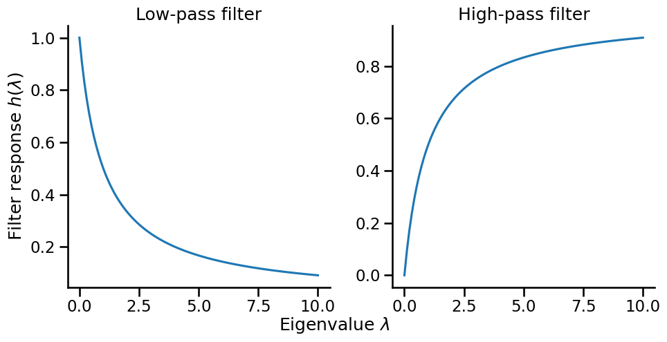
Eigenvalues $\lambda_i$ can be thought of as a filter that controls which frequency components pass through. Instead of using the filter associated with the Laplacian matrix, we can design a filter $h(\lambda_i)$ to control which frequency components pass through. This leads to the idea of spectral filtering. Two common filters are:

Low-pass Filter: $$h_{\text{low}}(\lambda) = \frac{1}{1 + \alpha\lambda}$$
- Preserves low frequencies (small λ)
- Suppresses high frequencies (large λ)
- Results in smoother signals
High-pass Filter: $$h_{\text{high}}(\lambda) = \frac{\alpha\lambda}{1 + \alpha\lambda}$$
- Preserves high frequencies
- Suppresses low frequencies
- Emphasizes differences between neighbors

../_images/bab48c820139b984a9b09b482bfb2dcc7192e67337a65f2e34844cff7a4a388d.png

Example#

Let us showcase the idea of spectral filtering with a simple example with the karate club network.

We will first compute the laplacian matrix and its eigendecomposition.

# Compute Laplacian matrix
deg = np.array(A.sum(axis=1)).reshape(-1)
D = sparse.diags(deg)
L = D - A

# Compute eigendecomposition
evals, evecs = np.linalg.eigh(L.toarray())

# Sort eigenvalues and eigenvectors
order = np.argsort(evals)
evals = evals[order]
evecs = evecs[:, order]

Now, let’s create a low-pass and high-pass filter.

alpha = 2
L_low = evecs @ np.diag(1 / (1 + alpha * evals)) @ evecs.T
L_high = evecs @ np.diag(alpha * evals / (1 + alpha * evals)) @ evecs.T

print("Size of low-pass filter:", L_low.shape)
print("Size of high-pass filter:", L_high.shape)

Size of low-pass filter: (34, 34)
Size of high-pass filter: (34, 34)

Notice that the high-pass filter and low-pass filter are matrices of the same size as the adjacency matrix $A$, which defines a ‘convolution’ on the graph as follows:

\[ {\bf x}' = {\bf L}_{\text{low}} {\bf x} \quad \text{or} \quad {\bf x}' = {\bf L}_{\text{high}} {\bf x}. \]

where ${\bf L}_{\text{low}}$ and ${\bf L}_{\text{high}}$ are the low-pass and high-pass filters, respectively, and ${\bf x}'$ is the convolved feature vector.

Now, let’s see how these filters work. Our first example is a random feature vector.

# Random feature vector
x = np.random.randn(A.shape[0], 1)

# Convolve with low-pass filter
x_low = L_low @ x

# Convolve with high-pass filter
x_high = L_high @ x

Let us visualize the results.

../_images/1ab814205970396008cd22b7bf2ec314397af0a09d98e12fea232ee8201d3309.png

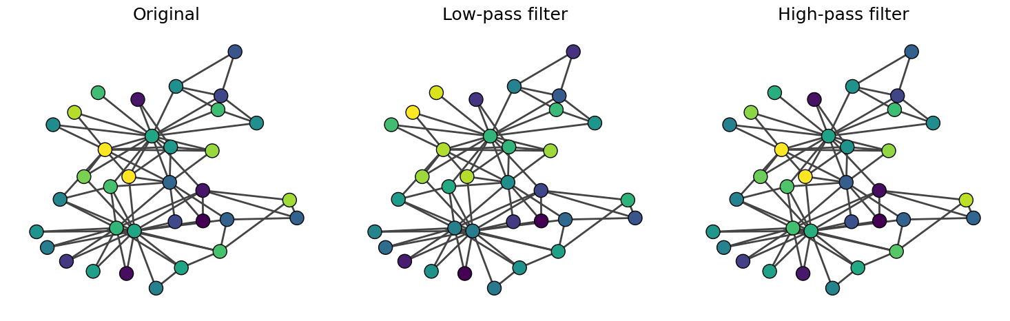
We observe that the low-pass filter results in smoother ${\bf x}$ between connected nodes (i.e., neighboring nodes have similar ${\bf x}$). The original ${\bf x}$ and ${\bf x}'_{\text{low}}$ are very similar because random variables are high-frequency components. In contrast, when we apply the high-pass filter, ${\bf x}'_{\text{high}}$ is similar to ${\bf x}$ because the high-frequency components are not filtered.

Let’s now use an eigenvector as our feature vector ${\bf x}$.

../_images/07eda8b148b6375def95d3d91ebe3fcb39cefda31d25866152362af8d7faf42b.png

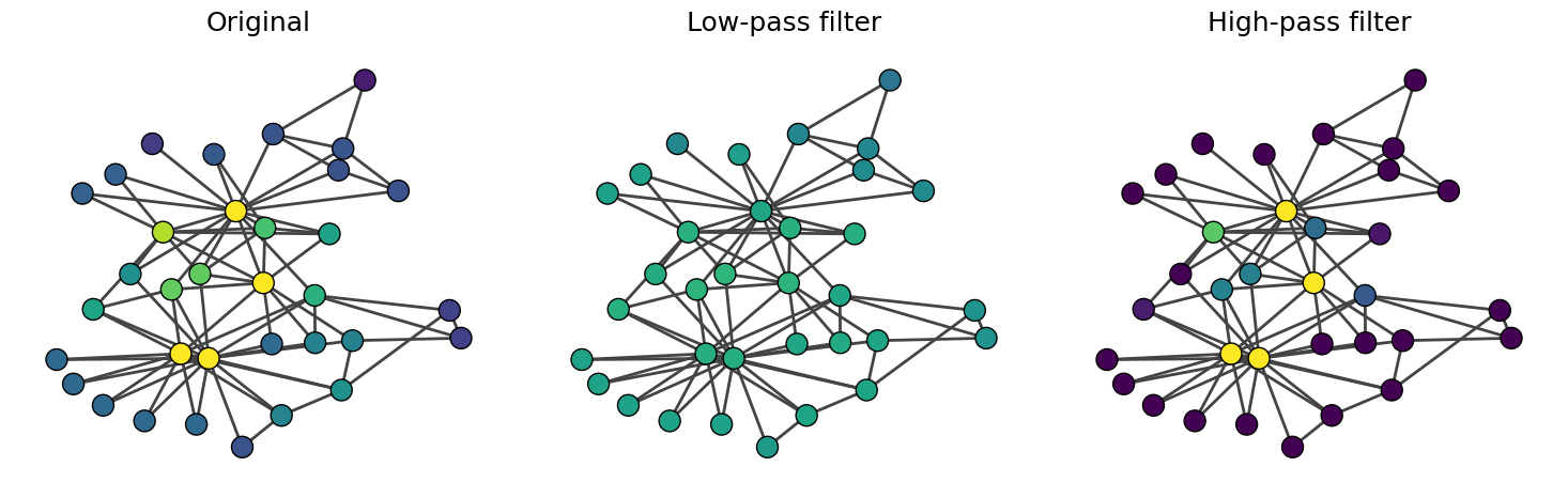
The high-pass filter increases the contrast of the eigenvector centrality, emphasizing the differences between nodes. On the other hand, the low-pass filter smooths out the eigenvector centrality.