VGGNet - A Deep Convolutional Neural Network for Image Recognition

VGGNet , introduced by Karen Simonyan and Andrew Zisserman from the Visual Geometry Group (VGG) at Oxford University, represents a significant milestone in the evolution of Convolutional Neural Networks (CNNs). At its core, VGGNet demonstrated that network depth is crucial for achieving superior performance in visual recognition tasks, a finding that would influence CNN design for years to come.

Tip

Historical Context: In 2014, when VGGNet secured victory at the ILSVRC challenge, the common belief was that deeper networks would be too difficult to train due to vanishing gradients and computational constraints. VGGNet’s success challenged this assumption and paved the way for even deeper architectures like ResNet.

Architecture

VGGNet employs a systematic stack of convolutional layers using exclusively 3×3 filters with stride 1 and padding 1, interspersed with 2×2 max pooling layers with stride 2. This uniformity makes the architecture conceptually simple.

Fig. 64 A schematic representation of VGG16 architecture showing the progression of spatial dimensions and feature channels through the network. The input is a 224×224×3 image, and the output is a 1000-dimensional vector for ImageNet classification. The image is taken from https://www.researchgate.net/profile/Max-Ferguson.

VGG has multiple variants, and the most popular one is VGG16, which has 16 layers. The full architecture of VGG16 is as follows:

• Input: [224 x 224] normalized, 3-channel color image (with color whitening, see section 3.2.1 in AlexNet article)

• Conv1_1: Convolutional layer - [3 x 3] kernel x 64 channels + ReLU

• Conv1_2: Convolutional layer - [3 x 3] kernel x 64 channels + ReLU

• P1: Pooling layer - Max pooling, [2 x 2] kernel, stride = 2

• Conv2_1: Convolutional layer - [3 x 3] kernel x 128 channels + ReLU

• Conv2_2: Convolutional layer - [3 x 3] kernel x 128 channels + ReLU

• P2: Pooling layer - Max pooling, [2 x 2] kernel, stride = 2

• Conv3_1: Convolutional layer - [3 x 3] kernel x 256 channels + ReLU

• Conv3_2: Convolutional layer - [3 x 3] kernel x 256 channels + ReLU

• Conv3_3: Convolutional layer - [1 x 1] kernel x 256 channels + ReLU

• P3: Pooling layer - Max pooling, [2 x 2] kernel, stride = 2

• Conv4_1: Convolutional layer - [3 x 3] kernel x 512 channels + ReLU

• Conv4_2: Convolutional layer - [3 x 3] kernel x 512 channels + ReLU

• Conv4_3: Convolutional layer - [1 x 1] kernel x 512 channels + ReLU

• P4: Pooling layer - Max pooling, [2 x 2] kernel, stride = 2

• Conv5_1: Convolutional layer - [3 x 3] kernel x 512 channels + ReLU

• Conv5_2: Convolutional layer - [3 x 3] kernel x 512 channels + ReLU

• Conv5_3: Convolutional layer - [1 x 1] kernel x 512 channels + ReLU

• P5: Pooling layer - Max pooling [7 x 7] kernel (aggressive downsampling at this stage)

• (During training only: Dropout)

• FC14: Fully connected layer - (7 x 7 x 512) → 4096

• (During training only: Dropout)

• FC15: Fully connected layer - 4096 → 4096

• FC16: Fully connected layer - 4096 → 1000

• Output: 1000-dimensional vector probability distribution (output probability for each dimension) using softmax function

The network progressively increases the number of feature channels after each pooling operation, following a clear doubling pattern:

\[ \text{channels} = \{64 \rightarrow 128 \rightarrow 256 \rightarrow 512 \rightarrow 512\} \]

The spatial dimensions of the feature maps decrease after each pooling layer, while the number of channels increases, creating a characteristic pyramid structure:

\[ \text{spatial dimensions} = \{224 \rightarrow 112 \rightarrow 56 \rightarrow 28 \rightarrow 14 \rightarrow 7\} \]

Despite its apparent simplicity, VGG16 contains approximately 140 million parameters, with the majority concentrated in the first fully connected layer (approximately 102 million parameters). This large parameter count highlights an interesting trade-off in the architecture: while the convolutional layers follow a clean and efficient design, the fully connected layers remain computationally intensive. This issue is later resolved by global average pooling proposed by [1].

Key Design Principles

The success of VGGNet stems from several key design principles that work in tandem to create a powerful yet conceptually simple architecture. These principles represent new best practices in CNN design. Let us examine each of these design choices and understand their theoretical foundations.

Parameter Reduction using Stacked 3x3 Kernels

One of the most influential contributions is the demonstration that stacking multiple 3×3 convolution layers can effectively replace larger kernels while reducing the total number of parameters. This principle is based on a fundamental insight about receptive fields in CNNs.

Consider that we stack two 3×3 convolution layers. Each value in the feature map of the first layer represents the summary of the 3×3 region of the input. The second layer then generates a new feature map by applying the same 3×3 convolution to the feature map of the first layer, summarizing the 5×5 region of the input. The receptive field of the second layer (i.e., the region of the input that the second layer can see) is 5×5.

Now, let us compare two cases:

1. A single 5×5 convolution layer with stride 1

2. Two stacked 3×3 convolution layers with stride 1

Which one has fewer parameters? The answer is the second case. In fact, a single 5×5 convolution layer has \(5 \times 5 =25\) parameters, while two stacked 3×3 convolution layers have \(2 \times (3 \times 3) = 18\) parameters.

This 28% reduction in parameters comes with an additional benefit: the inclusion of an extra ReLU non-linearity between the convolutions, allowing the network to be deeper.

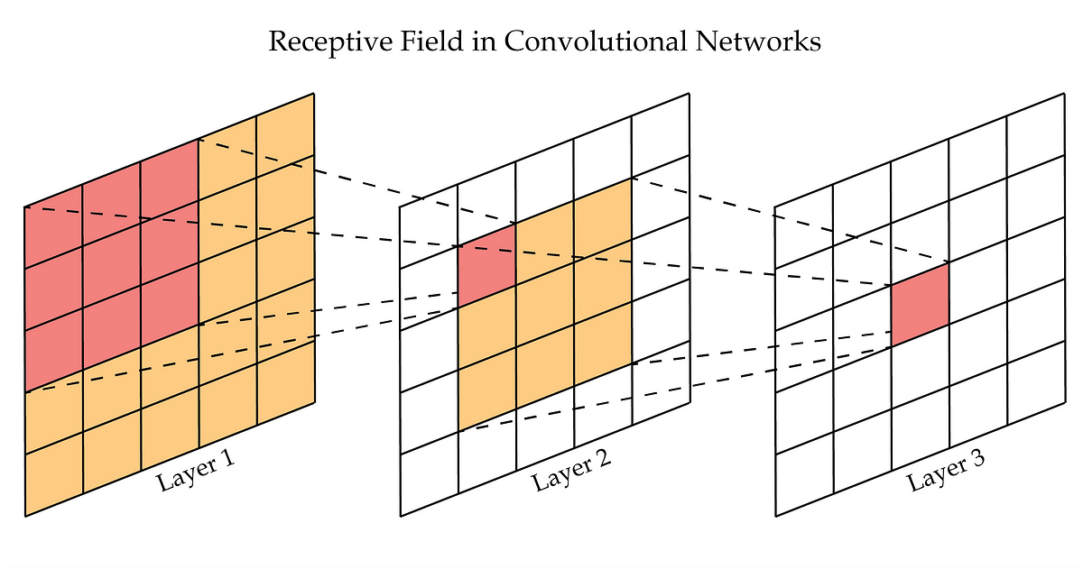
Fig. 65 A schematic representation of the receptive field of two stacked 3x3 convolution layers. The receptive field of the first layer is 3x3, and the receptive field of the second layer is 5x5. The image is taken from https://medium.com/@rekalantar/receptive-fields-in-deep-convolutional-networks-43871d2ef2e9

VGG-style Data Augmentation

VGGNet proposed multi-scale data augmentation (Figure 3). In AlexNet, data augmentation was performed by randomly cropping 224×224 input images from normalized images where the height was set to 256 pixels (left half of the figure below). In addition to this, VGGNet randomly crops 224×224 input images from images resized to a different scale with height of 384 pixels (right half of the figure below).

Through this VGGNet-style data augmentation approach of resizing to two scales, VGGNet was able to learn diversity across two scales, leading to improved classification accuracy.

Fig. 66 Data augmentation for VGGNet. The image is taken from https://cvml-expertguide.net/

[1]

Min Lin, Qiang Chen, and Shuicheng Yan. Network in network. CoRR, 2013. URL: https://api.semanticscholar.org/CorpusID:16636683.