Generative Pre-trained Transformer (GPT)

The Generative Pre-trained Transformer (GPT) [1] represents a significant evolution in transformer-based language models, focusing on powerful text generation capabilities through a decoder-only architecture. While BERT uses bidirectional attention to understand context, GPT employs unidirectional (causal) attention to generate coherent text by predicting one token at a time.

GPT in interactive notebook:

Here is a demo notebook for GPT

To run the notebook, download the notebook as a .py file and run it with:

marimo edit –sandbox gpt-interactive.py

You will need to install marimo and uv to run the notebook. But other packages will be installed automatically in uv’s virtual environment.

Architecture

Like in BERT, GPT also uses a transformer architecture. The main difference is that BERT uses an encoder transformer, while GPT uses a decoder transformer with some modifications.

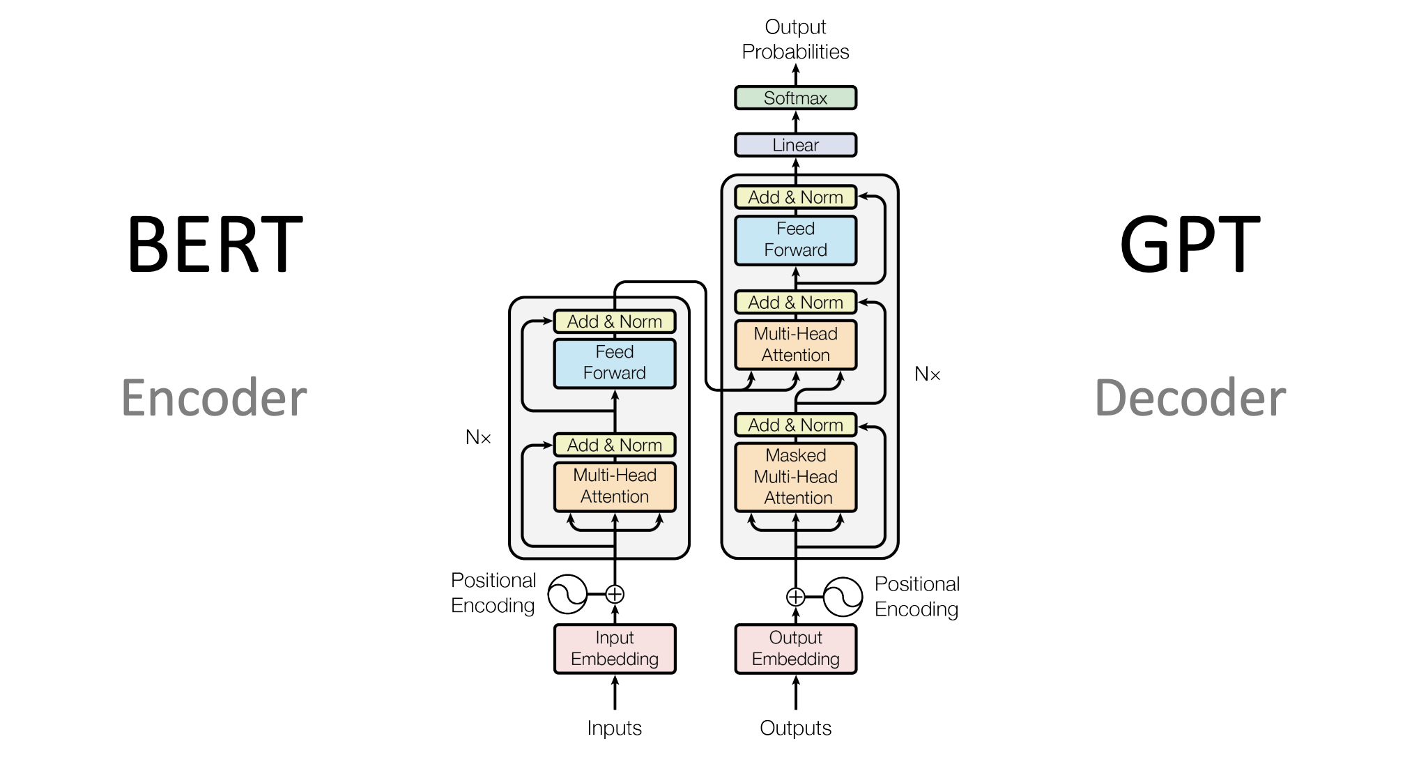
Fig. 35 GPT architecture.

Tip

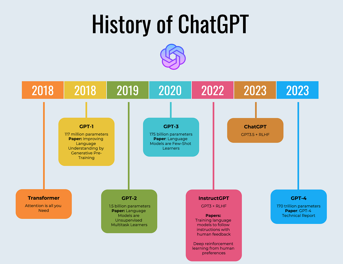
The GPT model family has evolved through several iterations, starting with GPT-1 in 2018 which introduced the basic architecture with 117M parameters and transfer learning capabilities. GPT-2 followed in 2019 with 1.5B parameters and zero-shot abilities, while GPT-3 in 2020 dramatically scaled up to 175B parameters, enabling few-shot learning. The latest GPT-4 (2023) features multimodal capabilities, improved reasoning, and a 32K token context window. Throughout these iterations, the core decoder-only transformer architecture remained unchanged, with improvements coming primarily from increased scale that enabled emergent capabilities.

Core Components

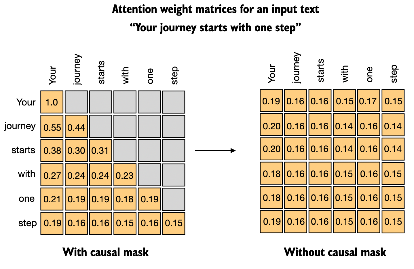
Fig. 36 Causal attention in GPT.

Like BERT, GPT uses learned token embeddings to convert input tokens into continuous vector representations. The model also employs learned positional embeddings that are added to the token embeddings to encode position information. A key difference from BERT is that GPT uses a causal attention mechanism, which means each position can only attend to previous positions in the sequence, enabling the model to generate text in a left-to-right fashion by predicting one token at a time.

Causal Language Modeling

Causal (autoregressive) language modeling is the pre-training objective of GPT, where the model learns to predict the next token given all previous tokens in the sequence. More formally, given a sequence of tokens \((x_1, x_2, ..., x_n)\), the model is trained to maximize the likelihood:

\[ P(x_1, ..., x_n) = \prod_{i=1}^n P(x_i|x_1, ..., x_{i-1}) \]

For example, given the partial sentence “The cat sat on”, the model learns to predict the next word by calculating probability distributions over its entire vocabulary. During training, it might learn that “mat” has a high probability in this context, while “laptop” has a lower probability.

Note

While BERT uses bidirectional attention and sees the entire sequence at once (making it powerful for understanding), GPT’s unidirectional approach more naturally models how humans write text, i.e., one word at a time, with each word influenced by all previous words. The bidirectional nature of BERT is more powerful for understanding, but it is less suitable for text generation.

Tip

The autoregressive nature of GPT means it’s particularly sensitive to the initial tokens (prompt) it receives. Well-crafted prompts that establish clear patterns or constraints can significantly improve generation quality.

The next-token prediction objective has remained unchanged across all GPT versions due to its remarkable effectiveness. Rather than modifying this core approach, improvements have come from increasing model size and refining the architecture. This simple yet powerful training method has become fundamental to modern language models.

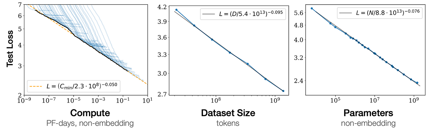
Scaling Laws

Language model performance improves predictably as models get larger, following simple mathematical relationships (power laws). The larger the model, the better it performs - and this improvement is reliable and measurable. This predictability was crucial for the development of models like GPT-3 and Claude, as it gave researchers confidence that investing in larger models would yield better results. Importantly, larger models are more efficient learners - they need proportionally less training data and fewer training steps to achieve good performance.

These findings revolutionized AI development by showing that better AI systems could be reliably built simply by scaling up model size, compute, and data in the right proportions. This insight led directly to the development of increasingly powerful models, as researchers could confidently invest in building larger and larger systems knowing they would see improved performance.

See the paper Scaling Laws for Neural Language Models for more details.

Inference Strategies

GPT does not generate text in one go. Instead, it predicts the next token repeatedly to generate text. GPT does not pick a specific token but provides a probability distribution over the next token. It is our job to sample a token from the distribution. There are several strategies to sample a token from the distribution as we will see below.

Fig. 37 GPT predicts the next token repeatedly to generate text.

Greedy and Beam Search

When generating text, language models assign probabilities to possible next tokens. Sampling a token from the distribution is not as easy as it might seem. This is because the distribution is high-dimensional. Namely, we need to sample a single token from millions of possible tokens, and thus, sampling a token can be computationally very expensive.

Greedy sampling always picks the highest probability token, which is deterministic but can lead to repetitive or trapped text. For example, if the model predicts “the” with high probability, it will always predict “the” again.

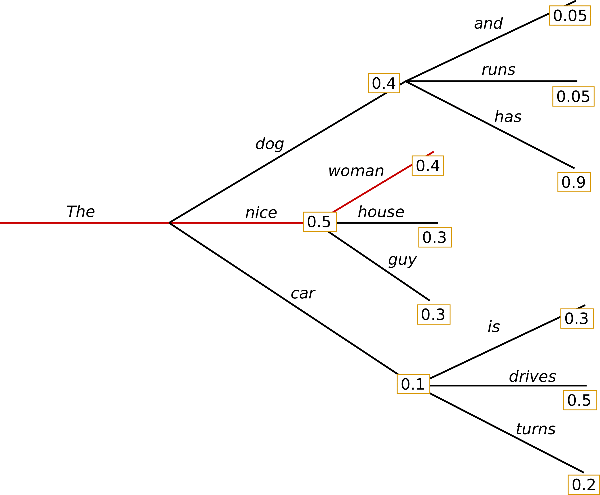
Fig. 38 GPT greedy search.

Beam search alleviates this problem by taking into account the high-order dependencies between tokens. For example, in generating “The cat ran across the ___”, beam search might preserve a path containing “mat” even if “floor” or “room” have higher individual probabilities at that position. This is because the complete sequence like “mat quickly” could be more probable when considering the token next after “mat”. “The cat ran across the mat quickly” is a more natural phrase than “The cat ran across the floor quickly” when considering the full flow and common linguistic patterns.

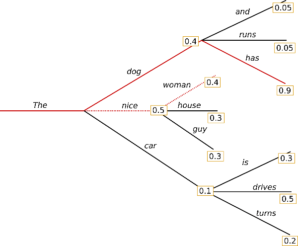
Fig. 39 GPT beam search.

Beam search maintains multiple possible sequences (beams) in parallel, exploring different paths simultaneously. At each step, it expands all current beams, scores the resulting sequences, and keeps only the top-k highest scoring ones. For instance, with a beam width of 3:

• First beams might be: [“The cat ran”, “The cat walked”, “The cat jumped”]

• Next step: [“The cat ran across”, “The cat ran through”, “The cat walked across”]

• And so on, keeping the 3 most promising complete sequences at each step

This process continues until reaching the end, finally selecting the sequence with highest overall probability. The beam search can be combined with top-k sampling or nucleus sampling. For example, one can sample a token based on the top-k sampling or nucleus sampling to form the next beam.

While beam search often produces high-quality outputs since it considers longer-term coherence, it can still suffer from the problem of repetitive or trapped text.

From Deterministic to Stochastic Sampling

Both greedy and beam search are deterministic. They pick the most likely token at each step. However, this creates a loop where the model always predicts the same tokens repeatedly. A simple way to alleviate this problem is to sample a token from the distribution.

Top-k Sampling relaxes the deterministic nature of greedy sampling by selecting randomly from the k most likely next tokens at each generation step. While this introduces some diversity compared to greedy sampling, choosing a fixed k can be problematic. Value of \(k\) might be too large for some distribution tails (including many poor options) or too small for others (excluding reasonable options).

Nucleus Sampling~[2] addresses this limitation by dynamically selecting tokens based on cumulative probability. It samples from the smallest set of tokens whose cumulative probability exceeds a threshold p (e.g. 0.9). This adapts naturally to different probability distributions, i.e., selecting few tokens when the distribution is concentrated and more when it’s spread out. This approach often provides a good balance between quality and diversity.

Fig. 40 Nucleus sampling. The image is taken from this blog.

Temperature Control Temperature (\(\tau\)) modifies how “concentrated” the probability distribution is for sampling by scaling the logits before applying softmax:

\[ p_i = \frac{\exp(z_i/\tau)}{\sum_j \exp(z_j/\tau)} \]

where \(z_i\) are the logits and \(\tau\) is the temperature parameter. Lower temperatures (\(\tau < 1.0\)) make the distribution more peaked, making high probability tokens even more likely to be chosen, leading to more focused and conservative outputs. Higher temperatures (\(\tau > 1.0\)) flatten the distribution by making the logits more similar, increasing the chances of selecting lower probability tokens and producing more diverse but potentially less coherent text. As \(\tau \to 0\), the distribution approaches a one-hot vector (equivalent to greedy search), while as \(\tau \to \infty\), it approaches a uniform distribution.

Fig. 41 Temperature controls the concentration of the probability distribution. Lower temperature makes the distribution more peaked, while higher temperature makes the distribution more flat.