AlexNet: A Breakthrough in Deep Learning

How can we train a computer to recognize 1000 different types of objects across more than a million images, and what makes this problem so challenging?

Conceptual Foundation: The ImageNet Challenge

Before diving into AlexNet, let’s explore why large-scale image classification posed such a formidable problem for machine learning:

1. Massive Dataset: The ImageNet Large Scale Visual Recognition Challenge (ILSVRC) dataset contains over 1.2 million training images labeled across 1000 categories.

2. Computational Demands: Traditional approaches struggled both with the sheer volume of data and with the complexity of designing handcrafted features.

3. Error Plateaus: Prior to 2012, the best error rates hovered around 25%, suggesting that existing methods had nearly peaked using conventional feature-engineering techniques.

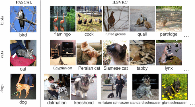
Fig. 59 The ImageNet Large Scale Visual Recognition Challenge (ILSVRC).

Tip

Prior to AlexNet, most computer vision systems relied on hand-engineered features such as SIFT (Scale-Invariant Feature Transform) or HOG (Histogram of Oriented Gradients). These were labor-intensive to design and often failed to generalize well to diverse images.

In 2012, a team led by Alex Krizhevsky, Ilya Sutskever, and Geoffrey Hinton demonstrated a deep Convolutional Neural Network (CNN) that shattered expectations. Their submission, known as AlexNet, reduced the top-5 error rate to 16.4%—a remarkable improvement of over 10 percentage points compared to the next-best approach [1].

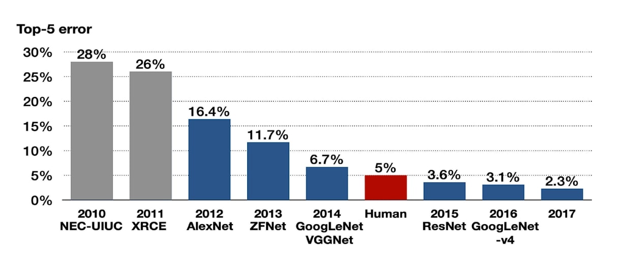
Fig. 60 Top 5 error rates of the ImageNet Large Scale Visual Recognition Challenge (ILSVRC) from 2010 to 2017. AlexNet reduced the error rate by over 10 percentage points compared to the best performing method based on human-crafted features in 2011.

This breakthrough ignited the deep learning revolution in computer vision. Researchers quickly realized the potential of stacking many layers of neural networks—provided they could overcome critical hurdles in training and regularization.

Key Innovations in AlexNet

ReLU Activation Function

The Challenge: Deep neural networks often suffer from the vanishing gradient problem, making early layers in the network extremely hard to train. Common activation functions like the sigmoid:

\[ \sigma(x) = \frac{1}{1 + e^{-x}} \]

suffer from saturation, where the gradient becomes almost zero if the input \(x\) is large (positive or negative).

The AlexNet Solution: Introduce the Rectified Linear Unit (ReLU) [2]:

\[ \text{ReLU}(x) = \max(0, x) \]

Fig. 61 Sigmoid vs. ReLU activation functions. Sigmoid can cause gradients to vanish for \(x\) far from zero, whereas ReLU maintains a constant gradient (1) for \(x>0\).

• Benefits:

  • Avoids vanishing gradients for positive \(x\).

  • Computationally efficient: Only a simple check if \(x>0\).

• Drawback:

  • Neurons can “die” (always output zero) if \(x\) stays negative. Variants like Leaky ReLU or Parametric ReLU (PReLU) introduce a small slope for \(x \leq 0\) to mitigate this.

Note

Leaky ReLU/PReLU are typically defined as:

\[\begin{split} f(x) = \begin{cases} x & \text{if } x > 0 \\ \alpha x & \text{if } x \leq 0 \end{cases} \end{split}\]

where \(\alpha\) is a small positive constant.

Dropout Regularization

Deep networks with millions of parameters can easily overfit to the training data, harming their ability to generalize.

The AlexNet solution is to use Dropout [3], a technique that randomly disables (or “drops out”) neurons with probability \(p\) during training.

Fig. 62 Dropout in action.

1. Training: Each neuron is “dropped” with probability \(p\), forcing the network to not rely on any single neuron’s output.

2. Inference: All neurons are used, but their outputs are scaled by \((1-p)\) to maintain expected values.

Note

An alternative known as inverse dropout scales weights by \(1/(1-p)\) during training, removing the need for scaling during inference. This is how many popular deep learning frameworks (e.g., TensorFlow) implement dropout.

---

3. Local Response Normalization (LRN)

In CNNs, neighboring feature maps can become disproportionately large, leading to unstable or less discriminative representations.

In the AlexNet, this is rectified by Local Response Normalization (LRN) , which normalizes activity across adjacent channels:

\[ b^i_{x,y} = \frac{a^i_{x,y}}{\Bigl(k + \alpha \sum_{j=\max(0,i-\frac{n}{2})}^{\min(N-1,i+\frac{n}{2})} (a^j_{x,y})^2\Bigr)^\beta} \]

Here, (a^i_{x,y}) is the activation at channel (i), and (k, \alpha, \beta, n) are constants. LRN encourages local competition among adjacent channels, akin to certain neural mechanisms in biological systems.

Note

LRN is less commonly used in modern architectures (like VGG, ResNet, etc.) which often rely on batch normalization or other normalization techniques. Still, LRN was a key component in AlexNet’s success at the time.

---

The AlexNet Architecture

Now that we’ve seen how AlexNet addressed vanishing gradients, overfitting, and feature-map normalization, let’s look at the overall blueprint:

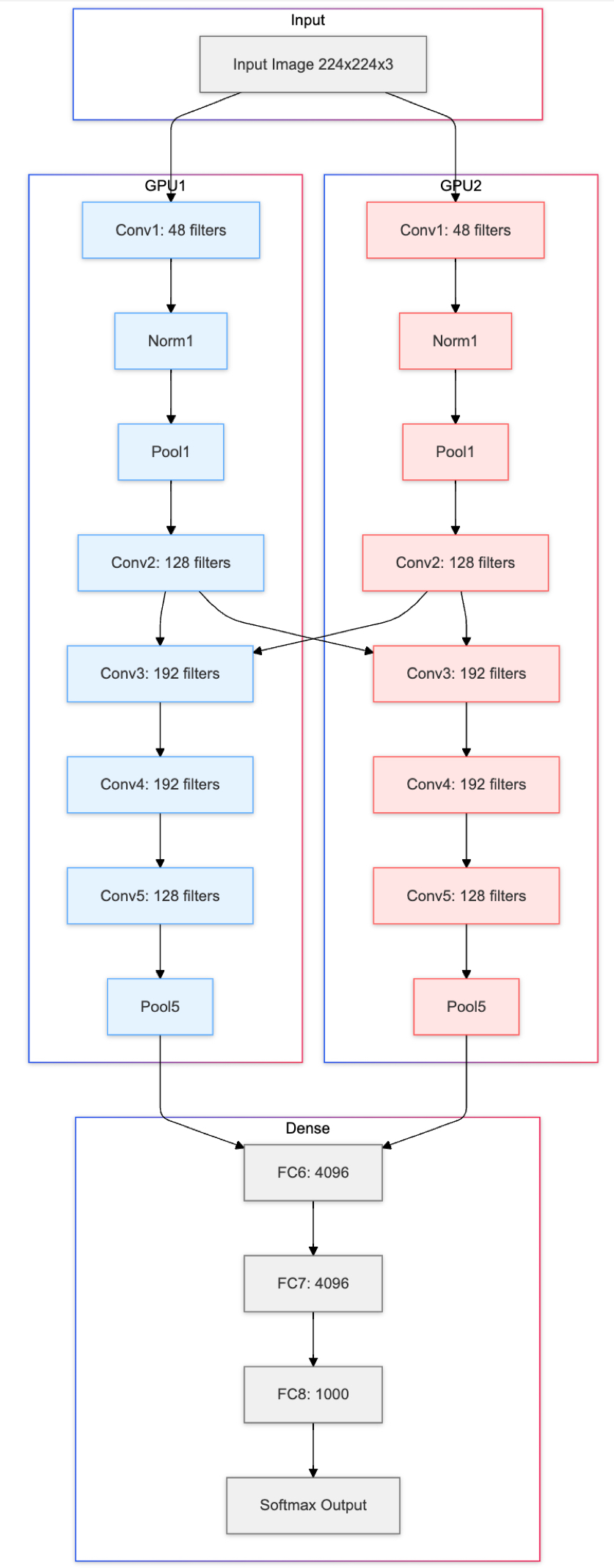
Fig. 63 A high-level view of the AlexNet architecture.

Detailed Layer-by-Layer Overview:

1. Input: 3-channel color image, 224×224 pixels

2. Conv1: [11×11, stride=4, padding=2] → ReLU → LRN → Overlapping Max Pool ([3×3], stride=2)

3. Conv2: [5×5, stride=1, padding=2] → ReLU → LRN → Overlapping Max Pool ([3×3], stride=2)

4. Conv3: [3×3, stride=1, padding=1] → ReLU

5. Conv4: [3×3, stride=1, padding=1] → ReLU

6. Conv5: [3×3, stride=1, padding=1] → ReLU → Overlapping Max Pool ([3×3], stride=2)

7. FC6: Flatten → 9216 → 4096 → ReLU → Dropout

8. FC7: 4096 → 4096 → ReLU → Dropout

9. FC8: 4096 → 1000 → Softmax Output

Tip

Parallel GPU Computation AlexNet was trained on two GPUs with 3GB of memory each, splitting feature maps between them to handle the large parameter count. This approach showcased the necessity and practicality of GPU computing for large-scale deep learning.

---

Implementation Example

Below is a minimal snippet illustrating how one might instantiate an AlexNet-like model using PyTorch’s built-in module. For a step-by-step tutorial, check out Writing AlexNet from Scratch in PyTorch | DigitalOcean.

import torch
import torch.nn as nn
import torch.nn.functional as F

class SimpleAlexNet(nn.Module):
    def __init__(self, num_classes=1000):
        super(SimpleAlexNet, self).__init__()
        self.features = nn.Sequential(
            nn.Conv2d(3, 96, kernel_size=11, stride=4, padding=2),
            nn.ReLU(inplace=True),
            # LRN is omitted in modern PyTorch models, replaced by batch norm or left out
            nn.MaxPool2d(kernel_size=3, stride=2),

            nn.Conv2d(96, 256, kernel_size=5, padding=2),
            nn.ReLU(inplace=True),
            # Another LRN placeholder if needed
            nn.MaxPool2d(kernel_size=3, stride=2),

            nn.Conv2d(256, 384, kernel_size=3, padding=1),
            nn.ReLU(inplace=True),

            nn.Conv2d(384, 384, kernel_size=3, padding=1),
            nn.ReLU(inplace=True),

            nn.Conv2d(384, 256, kernel_size=3, padding=1),
            nn.ReLU(inplace=True),
            nn.MaxPool2d(kernel_size=3, stride=2),
        )

        self.classifier = nn.Sequential(
            nn.Dropout(),
            nn.Linear(256 * 6 * 6, 4096),
            nn.ReLU(inplace=True),
            nn.Dropout(),
            nn.Linear(4096, 4096),
            nn.ReLU(inplace=True),
            nn.Linear(4096, num_classes),
        )

    def forward(self, x):
        x = self.features(x)
        x = torch.flatten(x, 1)
        x = self.classifier(x)
        return x

# Instantiate the model
model = SimpleAlexNet(num_classes=1000)
print(model)

SimpleAlexNet(
  (features): Sequential(
    (0): Conv2d(3, 96, kernel_size=(11, 11), stride=(4, 4), padding=(2, 2))
    (1): ReLU(inplace=True)
    (2): MaxPool2d(kernel_size=3, stride=2, padding=0, dilation=1, ceil_mode=False)
    (3): Conv2d(96, 256, kernel_size=(5, 5), stride=(1, 1), padding=(2, 2))
    (4): ReLU(inplace=True)
    (5): MaxPool2d(kernel_size=3, stride=2, padding=0, dilation=1, ceil_mode=False)
    (6): Conv2d(256, 384, kernel_size=(3, 3), stride=(1, 1), padding=(1, 1))
    (7): ReLU(inplace=True)
    (8): Conv2d(384, 384, kernel_size=(3, 3), stride=(1, 1), padding=(1, 1))
    (9): ReLU(inplace=True)
    (10): Conv2d(384, 256, kernel_size=(3, 3), stride=(1, 1), padding=(1, 1))
    (11): ReLU(inplace=True)
    (12): MaxPool2d(kernel_size=3, stride=2, padding=0, dilation=1, ceil_mode=False)
  )
  (classifier): Sequential(
    (0): Dropout(p=0.5, inplace=False)
    (1): Linear(in_features=9216, out_features=4096, bias=True)
    (2): ReLU(inplace=True)
    (3): Dropout(p=0.5, inplace=False)
    (4): Linear(in_features=4096, out_features=4096, bias=True)
    (5): ReLU(inplace=True)
    (6): Linear(in_features=4096, out_features=1000, bias=True)
  )
)

In practice, PyTorch provides a pre-trained version of AlexNet via torchvision.models.alexnet. You can load it with:

import torchvision.models as models
alexnet = models.alexnet(pretrained=True)

/Users/skojaku-admin/miniforge3/envs/applsoftcomp/lib/python3.10/site-packages/torchvision/models/_utils.py:208: UserWarning: The parameter 'pretrained' is deprecated since 0.13 and may be removed in the future, please use 'weights' instead.
  warnings.warn(
/Users/skojaku-admin/miniforge3/envs/applsoftcomp/lib/python3.10/site-packages/torchvision/models/_utils.py:223: UserWarning: Arguments other than a weight enum or `None` for 'weights' are deprecated since 0.13 and may be removed in the future. The current behavior is equivalent to passing `weights=AlexNet_Weights.IMAGENET1K_V1`. You can also use `weights=AlexNet_Weights.DEFAULT` to get the most up-to-date weights.
  warnings.warn(msg)

[1]

Alex Krizhevsky, Ilya Sutskever, and Geoffrey E Hinton. Imagenet classification with deep convolutional neural networks. In F. Pereira, C.J. Burges, L. Bottou, and K.Q. Weinberger, editors, Advances in Neural Information Processing Systems, volume 25. Curran Associates, Inc., 2012. URL: https://proceedings.neurips.cc/paper_files/paper/2012/file/c399862d3b9d6b76c8436e924a68c45b-Paper.pdf.

[2]

Vinod Nair and Geoffrey E. Hinton. Rectified linear units improve restricted boltzmann machines. In Proceedings of the 27th International Conference on International Conference on Machine Learning, ICML’10, 807–814. Madison, WI, USA, 2010. Omnipress.

[3]

Nitish Srivastava, Geoffrey Hinton, Alex Krizhevsky, Ilya Sutskever, and Ruslan Salakhutdinov. Dropout: a simple way to prevent neural networks from overfitting. The journal of machine learning research, 15(1):1929–1958, 2014.