From Traditional Image Processing to Learning

Image is a 2D matrix that can be extremely large. For example, a 1024x1024 image has 1,048,576 pixels. Processing such a high-dimensional data with neural networks requires a large number of parameters, the prohibitive computational cost, and an enormous dataset for training.

Convolutional Neural Networks (CNNs) were developed to address this key limitation of fully connected networks by leveraging convolution operation that leverages the local connectivity. Namely, instead of processing the entire image, CNN only processes a small region of the image at a time, and progressively integrates the information from the local regions to form a global representation. Here, we will first introduce the building blocks of CNNs, and then discuss how CNNs are built upon these blocks.

Building block of CNNs

Convolutional Layer

At the heart of Convolutional Neural Networks (CNNs) lies a remarkably elegant operation called convolution. Imagine sliding a small window, called a kernel or filter, across an image. At each position, we perform a simple multiplication and addition operation between the kernel values and the overlapping image pixels. This fundamental operation allows CNNs to automatically learn and detect important visual features.

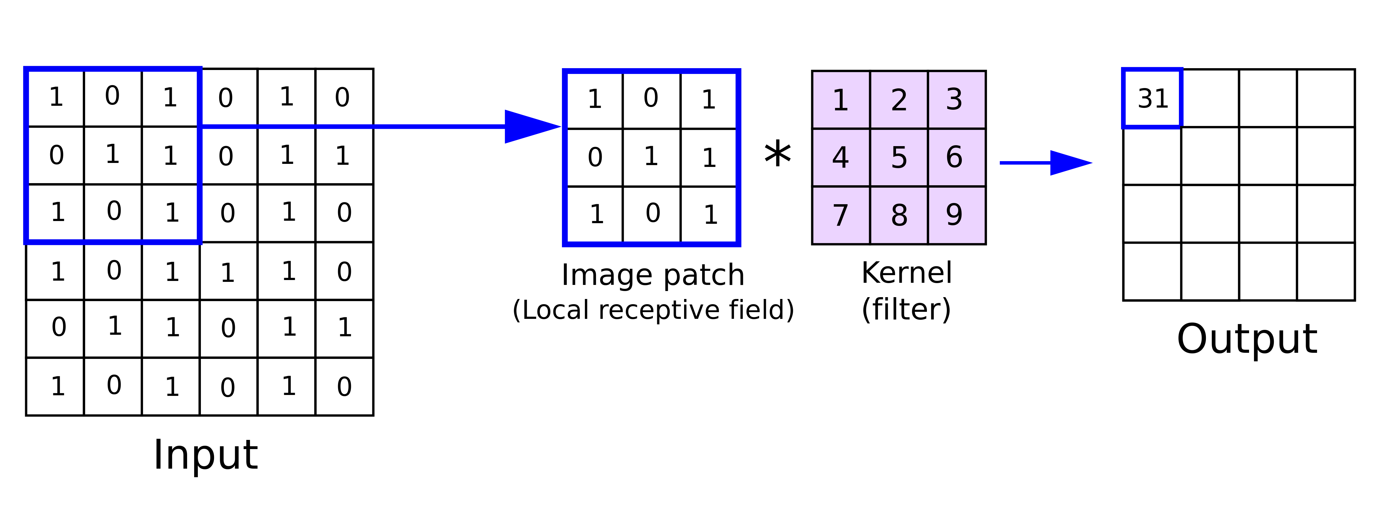
Fig. 50 Convolution operation. The kernel slides across the input image and performs the multiplication and addition operation at each position. The result is a feature map that represents the detected features. Image taken from https://anhreynolds.com/blogs/cnn.html

Let’s understand this mathematically. For a single-channel input (like a grayscale image), the 2D convolution operation can be expressed as:

\[ (I * K)_{i,j} = \sum_{m=0}^{L-1}\sum_{n=0}^{L-1} I_{i+m,j+n} \cdot K_{m,n} \]

where \(I\) represents the input image, \(K\) is the kernel, and \(*\) denotes the convolution operation. The indices \(i,j\) represent the position in the output feature map, while \(m,n\) traverse the kernel dimensions of size \(L\).

What makes CNNs powerful is that these kernels are learnable parameters. During training, each kernel evolves to detect specific visual patterns. Some kernels might become edge detectors, highlighting vertical or horizontal edges, while others might respond to textures or more complex patterns. This hierarchical feature learning is what makes CNNs so effective at visual recognition tasks.

Real-world images typically have multiple channels (like RGB). The convolution operation naturally extends to handle this by using 3D kernels. For an input with \(C\) channels, the operation becomes:

\[ (I * K)_{i,j} = \sum_{c=1}^{C}\sum_{m=0}^{L-1}\sum_{n=0}^{L-1} I_{c,i+m,j+n} \cdot K_{c,m,n} \]

where \(I\) is a 3D matrix with the last dimension of size \(C\), and \(K\) is a 3D kernel with the last dimension of size \(C\) as well. \(C\) is the number of channels in the input image.

Fig. 51 Convolution operation for multi-channel input. Each channel is processed separately, and the results are summed up to produce the final output.

Tip

Interactive visualization of convolution neural networks

• An Interactive Node-Link Visualization of Convolutional Neural Networks

• CNN Explainer

One of the key features of CNNs is translation equivariance. This means that when an input image is shifted, the output feature map shifts by the same amount. For example, if we move an object in an image one pixel to the right, its detected features in the output will also move one pixel to the right. This property allows CNNs to detect features consistently regardless of their position in the image.

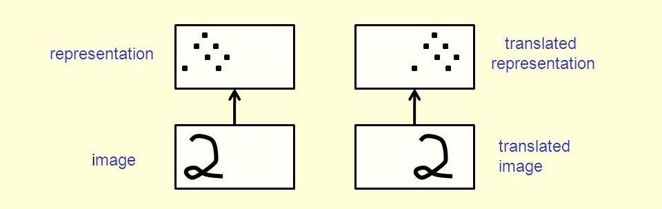
Fig. 52 Translation invariance. The same kernel can detect the same feature regardless of its position in the input.

Another key feature of convolutional layers is parameter sharing. Unlike dense neural networks where each parameter is used only once, a kernel’s weights are reused as it slides across the input. For example, a 3×3 kernel applied to a 224×224 RGB image (i.e., 3 channels) uses just 27 parameters (3×3×3) instead of the millions required by a fully connected layer. This weight-sharing scheme not only drastically reduces the model’s parameter count but also preserves spatial relationships in the data.

Receptive Field is the region of input pixels that influence each output pixel. This field grows larger in deeper layers through the combination of convolution and pooling, allowing CNNs to detect increasingly complex, hierarchical, and abstract features. For example, the first layer might detect edges, while deeper layers might recognize complex patterns like faces or objects.

Fig. 53 Receptive field of each convolution layer with a 3x3 kernel. The green area marks the receptive field of each layer. The image is taken from https://www.mdpi.com/2072-4292/9/5/480

Stride and Padding

In convolutional networks, stride and padding are crucial hyperparameters that control how we process spatial information. Stride (\(S\)) determines how many pixels we skip when sliding our kernel across the input. With stride-1, we move the kernel one pixel at a time, creating dense feature maps. When we increase the stride to 2 or more, we take larger steps, effectively downsampling the input. For a one-dimensional example, consider an input signal \([a,b,c,d,e,f]\) and a kernel \([1,2]\). With stride-1, we compute: $\( \begin{aligned} &[1a + 2b, \ &\phantom{[}1b + 2c, \ &\phantom{[}1c + 2d, \ &\phantom{[}1d + 2e, \ &\phantom{[}1e + 2f] \end{aligned} \)$

However, with stride-2, we skip every other position: $\( [1a + 2b, 1c + 2d, 1e + 2f] \)$ This striding mechanism serves two purposes: it reduces computational complexity and increases the receptive field (the region of input pixels that influence each output pixel).

Fig. 54 Stride-1 and stride-2. The image is taken from https://svitla.com/blog/math-at-the-heart-of-cnn/

Tip

Interactive visualization of stride

• Convolution Visualizer

Padding addresses a different challenge: information loss at the borders. Without padding (“valid” padding), the output dimensions shrink after each convolution because the kernel can’t fully overlap with border pixels. While various padding schemes are proposed, zero padding has been widely used because it is simple and effective.

Fig. 55 Padding. The image is taken from https://svitla.com/blog/math-at-the-heart-of-cnn/

Mathematically, for a square input of size \(W\) with kernel size \(K\), stride \(S\), and padding \(P\), the output dimension \(O\) is given by: $\( O = \left\lfloor\frac{W - K + 2P}{S}\right\rfloor + 1 \)$ Let’s break this formula down:

• \(W - K\) represents how far the kernel can move

• \(2P\) accounts for padding on both sides

• Division by \(S\) reflects the stride’s effect

• The floor function \(\lfloor \cdot \rfloor\) ensures integer output

• Adding 1 accounts for the initial position

For example, with an input size of 224×224, a 3×3 kernel, stride-2, and padding-1: $\( O = \left\lfloor\frac{224 - 3 + 2(1)}{2}\right\rfloor + 1 = 112 \)$

The interplay between stride and padding allows network designers to control information flow and computational efficiency. Larger strides create more compact representations but might miss fine details, while appropriate padding ensures no spatial information is unnecessarily discarded.

Note

Try out CNN Explainer to learn how convolution, padding, and stride affect the output.

Pooling Layer

Pooling layers serve as the dimensionality reduction modules in CNNs, summarizing spatial regions into single values while preserving essential features. Max-pooling, for example, is a widely used pooling operation that selects the highest activation value within a local region. For a feature map \(F\) (i.e., intermediate representation of a convolutional layer), max pooling over a 3×3 window can be expressed as:

\[ P_{i,j} = \max_{m=0,1}\max_{n=0,1} F_{3i+m,3j+n} \]

Max-pooling offers several key benefits. First, it creates a form of local translation invariance - small shifts in feature positions are absorbed by the pooling window. For instance, if an edge moves slightly within a 2×2 pooling region, the max-pooled output remains unchanged. Second, by reducing spatial dimensions, pooling significantly decreases computational complexity in subsequent layers.

Similarly, average pooling computes:

\[ P_{i,j} = \frac{1}{9}\sum_{m=0}^2\sum_{n=0}^2 F_{3i+m,3j+n} \]

The output dimensions after a pooling operation follow a similar formula to strided convolutions, but without padding considerations:

\[ O = \left\lfloor\frac{W - K}{S}\right\rfloor + 1 \]

where \(W\) is the input size, \(K\) is the pooling window size (typically 2 or 3), and \(S\) is the stride (usually equal to \(K\)).

Tip

Modern CNN architectures often debate the necessity of pooling layers [1]. Some networks replace them with strided convolutions, arguing that learnable downsampling might be more effective. The key difference lies in parameterization - pooling has no learnable parameters, while strided convolutions learn how to downsample. Consider these approaches:

\[ \text{Max Pooling: } y = \max(x_1, x_2, x_3, x_4) \]

\[ \text{Strided Conv: } y = w_1x_1 + w_2x_2 + w_3x_3 + w_4x_4 \]

Despite this trend, pooling layers remain valuable in many applications. They offer built-in invariance to small translations and rotations, reduce overfitting through their parameter-free nature, and provide consistent dimension reduction.

[1]

Jost Tobias Springenberg, Alexey Dosovitskiy, Thomas Brox, and Martin A. Riedmiller. Striving for simplicity: the all convolutional net. In Yoshua Bengio and Yann LeCun, editors, 3rd International Conference on Learning Representations, ICLR 2015, San Diego, CA, USA, May 7-9, 2015, Workshop Track Proceedings. 2015. URL: http://arxiv.org/abs/1412.6806.