import torch
from transformers import AutoModel, AutoTokenizer
import matplotlib.pyplot as plt
import seaborn as sns

# Load a small BERT model
model_name = "bert-base-uncased"
tokenizer = AutoTokenizer.from_pretrained(model_name)
model = AutoModel.from_pretrained(model_name, output_attentions=True)

text = "The bank of the river."
inputs = tokenizer(text, return_tensors="pt")
outputs = model(**inputs)

# Get attention from the last layer
# Shape: (batch, heads, seq_len, seq_len)
attention = outputs.attentions[-1].squeeze(0)

# Average attention across all heads for simplicity
mean_attention = attention.mean(dim=0).detach().numpy()
tokens = tokenizer.convert_ids_to_tokens(inputs["input_ids"][0])

# Plot
plt.figure(figsize=(8, 6))
sns.heatmap(mean_attention, xticklabels=tokens, yticklabels=tokens, cmap="viridis")
plt.title("BERT Attention Map (Last Layer)")
plt.xlabel("Key (Source)")
plt.ylabel("Query (Target)")
plt.show()BERT, GPT, and Sentence Transformers
What you’ll learn in this module
BERT and GPT are not variants of one architecture. They represent fundamentally different information flows.
You’ll learn:
- What makes BERT and GPT fundamentally different architectures, and why bidirectional vs. causal attention determines what each model can learn.
- How BERT’s encoder stack sees everything at once for deep understanding, while GPT’s decoder stack processes text sequentially for generation.
- The training objectives that shape these models: Masked Language Modeling (MLM) and Next Sentence Prediction (NSP) for BERT, versus Causal Language Modeling (CLM) for GPT.
- How to visualize attention patterns to understand what BERT learns about word relationships.
Two Siblings, BERT and GPT

We instinctively think of “Transformers” as a single unified model, but this is wrong. The original Transformer paper proposed an Encoder-Decoder architecture, a two-part machine. Modern models split this architecture in half, creating two distinct lineages with fundamentally different information flows.
BERT (Bidirectional Encoder Representations from Transformers) uses the encoder stack and sees everything at once, like reading a completed sentence. GPT (Generative Pre-trained Transformer) uses the decoder stack and processes text causally, like improvising a story where you can only react to what’s already been said. This architectural choice determines what the model can learn and what tasks it excels at.
Think of it like two different reading strategies: BERT is the student who reads the entire paragraph, then goes back to understand each word in context, while GPT is the actor performing a cold read, processing each line sequentially without peeking ahead at the script. The first strategy gives deeper understanding, the second gives the ability to continue the story.
Architecture
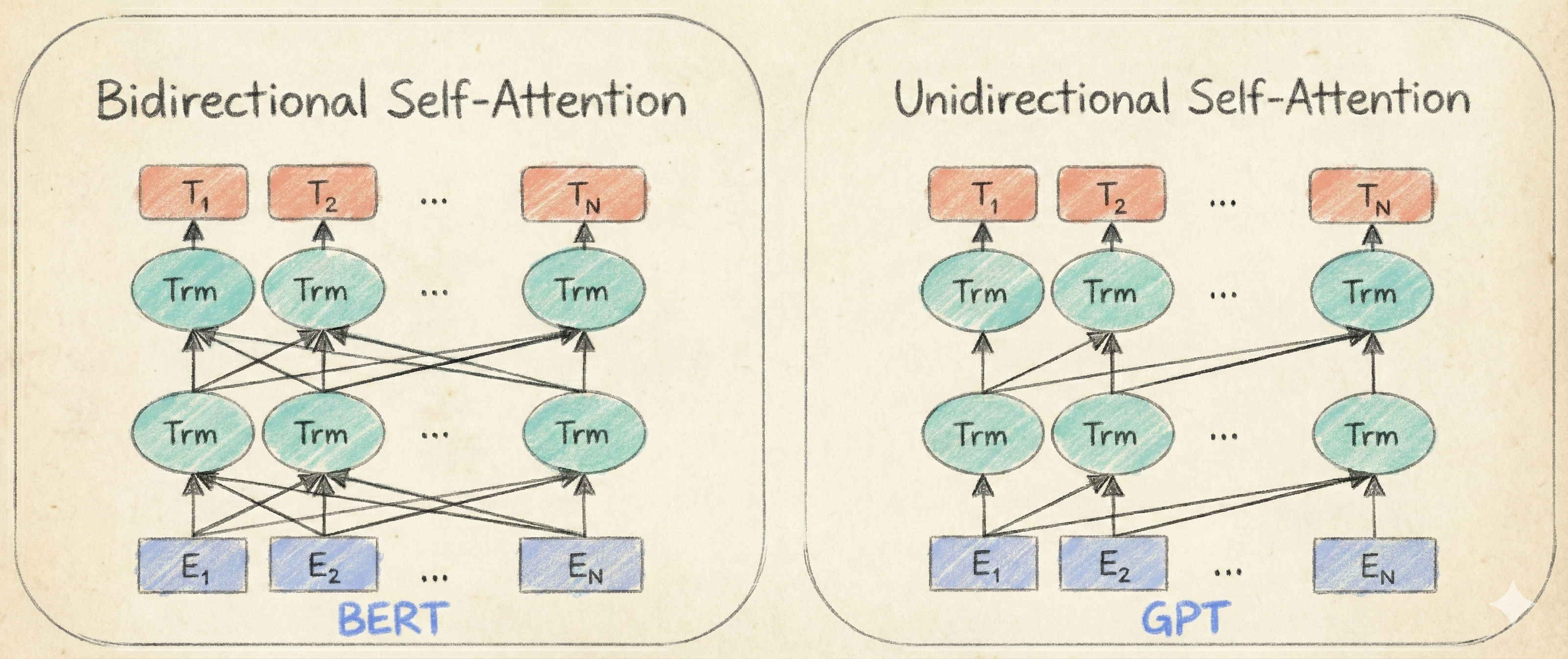
What’s the most important difference? The attention mechanism. BERT uses bidirectional attention, meaning every token at position t can attend to every other token. This allows BERT to understand the context of a word by looking at all the words in the sentence, capturing full context.
GPT uses masked (or causal) attention, meaning a token at position t can only attend to previous tokens. This masking imposes a causal constraint, making it ideal for language generation where the model must predict future tokens based only on past context. Although less globally context-aware than BERT, this causal processing allows GPT to generate remarkably fluent and coherent text sequentially.
More on BERT
Let’s talk about BERT’s special tokens. The [CLS] token represents the start of the sentence, [SEP] marks sentence boundaries, [MASK] represents masked words, and [UNK] represents unknown words. For example, the sentence “The cat sat on the mat. It then went to sleep.” becomes “[CLS] The cat sat on the mat [SEP] It then went to sleep [SEP]”.
Why does the [CLS] token matter? BERT learns to encode a summary of the input into the [CLS] token, making it particularly useful when we want the embedding of the whole input text rather than token-level embeddings.
BERT uses position and segment embeddings to provide contextual information. Unlike the sinusoidal position embedding used in the original transformer paper, BERT uses learnable position embeddings. Segment embeddings distinguish sentences in the input: tokens in the first sentence receive segment embedding 0, tokens in the second receive segment embedding 1. Both types of embeddings are learned during pre-training.
Several BERT variants have been developed. RoBERTa (Robustly Optimized BERT Approach) improved upon BERT by removing Next Sentence Prediction, using dynamic masking, training with larger batches and datasets, leading to significant performance improvements. DistilBERT focused on efficiency through knowledge distillation, achieving 95% of BERT’s performance while being 40% smaller and 60% faster. ALBERT introduced parameter reduction techniques using factorized embedding parameterization and cross-layer parameter sharing while replacing NSP with Sentence Order Prediction.
Domain-specific BERT models have been trained on specialized corpora for specific fields (BioBERT for biomedical text, SciBERT for scientific papers, FinBERT for financial documents), demonstrating superior performance in their respective domains. Multilingual BERT (mBERT) was trained on Wikipedia data from 104 languages and shows remarkable zero-shot cross-lingual transfer abilities despite lacking explicit cross-lingual objectives, making it valuable for low-resource languages.
Training
BERT
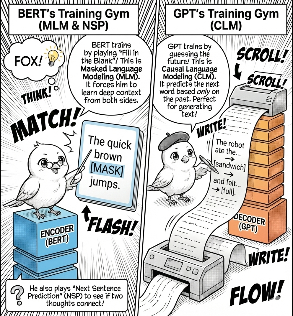
How do you train models with such different architectures? BERT, with its encoder-only design, is trained using two primary unsupervised tasks: Masked Language Modeling (MLM) and Next Sentence Prediction (NSP).
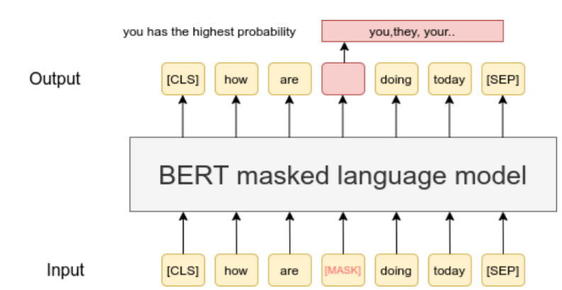
In MLM, a percentage of input tokens are randomly masked, and the model predicts the original tokens based on full bidirectional context. For example, given “The quick brown fox jumps over the lazy dog,” BERT might see “The quick brown [MASK] jumps over the lazy dog” and predict “fox.”
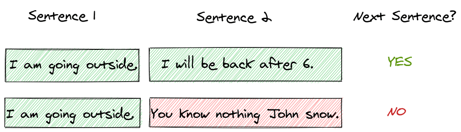
NSP involves presenting the model with two sentences and asking it to predict whether the second sentence logically follows the first. Given “The cat sat on the mat.” followed by “It was a sunny day.”, BERT would predict ‘IsNextSentence = No’, but for “It was purring softly.”, BERT would predict ‘IsNextSentence = Yes’. These tasks enable BERT to learn deep contextual representations for understanding text.
Recipe for MLM
To generate training data for MLM, BERT randomly masks 15% of the tokens in each sequence. The masking strategy uses three approaches: 80% of the time, replace the word with [MASK] (“the cat sat on the mat” becomes “the cat [MASK] on the mat”), 10% of the time, replace with a random word (“the cat dog on the mat”), and 10% of the time, keep unchanged (“the cat sat on the mat”).
Why this strange mix? The model must predict the original token for all selected positions regardless of how they were modified, preventing the model from simply learning to detect replaced tokens. During training, the model processes the modified sequence through its transformer layers and predicts the original token at each masked position using contextual representations. This approach, while counterintuitive, has proven effective and become essential to BERT’s pre-training.
Recipe for NSP
Next Sentence Prediction (NSP) trains BERT to understand relationships between sentences by predicting whether two sentences naturally follow each other. During training, half of the pairs are consecutive sentences from documents (labeled IsNext), the other half are random pairs (labeled NotNext).
The input format uses special tokens: [CLS] at the start, the first sentence, [SEP], the second sentence, and a final [SEP]. For instance:
\text{``[CLS] }\underbrace{\text{I went to the store}}_{\text{Sentence 1}}\text{ [SEP] }\underbrace{\text{They were out of milk}}_{\text{Sentence 2}}\text{ [SEP]''}.
BERT uses the final hidden state of the [CLS] token to classify whether the sentences are consecutive, helping the model develop broader understanding of language context and relationships.
GPT
What about GPT? GPT uses its decoder-only architecture for Causal Language Modeling (CLM), where the model learns to predict the next token given all previous tokens. More formally, given a sequence (x_1, x_2, ..., x_n), the model maximizes:
P(x_1, ..., x_n) = \prod_{i=1}^n P(x_i|x_1, ..., x_{i-1})
For example, given “The cat sat on”, the model calculates probability distributions over its vocabulary: “mat” might have high probability while “laptop” has lower probability. This autoregressive nature means GPT processes text left to right, learning to generate coherent and grammatically correct continuations that directly align with its strength in text generation.
Visualizing Attention: What Is BERT Looking At?
BERT produces attention weights, a matrix showing which tokens influence each other. We can extract these weights and visualize them to understand how the model disambiguates meaning.
In this heatmap, a bright spot at row “bank” and column “river” reveals that BERT is using “river” to understand “bank”, disambiguating it from a financial institution. This bidirectional flow is why BERT excels at tasks requiring deep contextual understanding like question answering and named entity recognition.
The Takeaway
BERT reads to understand. GPT writes to create. Choose the architecture that matches your information flow: bidirectional for deep contextual analysis, causal for sequential generation.