This section transforms you into a CNN practitioner.
You’ll learn:
What convolution operations do and how learnable kernels detect visual patterns.
The key properties of translation equivariance and parameter sharing that make CNNs efficient.
How receptive fields grow with depth and why this enables hierarchical feature learning.
The role of stride, padding, and pooling in controlling dimensions and creating invariance.
How to use pre-trained models from torchvision for immediate image classification.
Two approaches to transfer learning: feature extraction and fine-tuning for custom tasks.
Understanding CNN Building Blocks
AlexNet proved that deep learning works at scale, but how do these networks actually process images? Let’s break down the fundamental operations that make CNNs powerful.
Convolutional Layers: Learnable Pattern Detectors
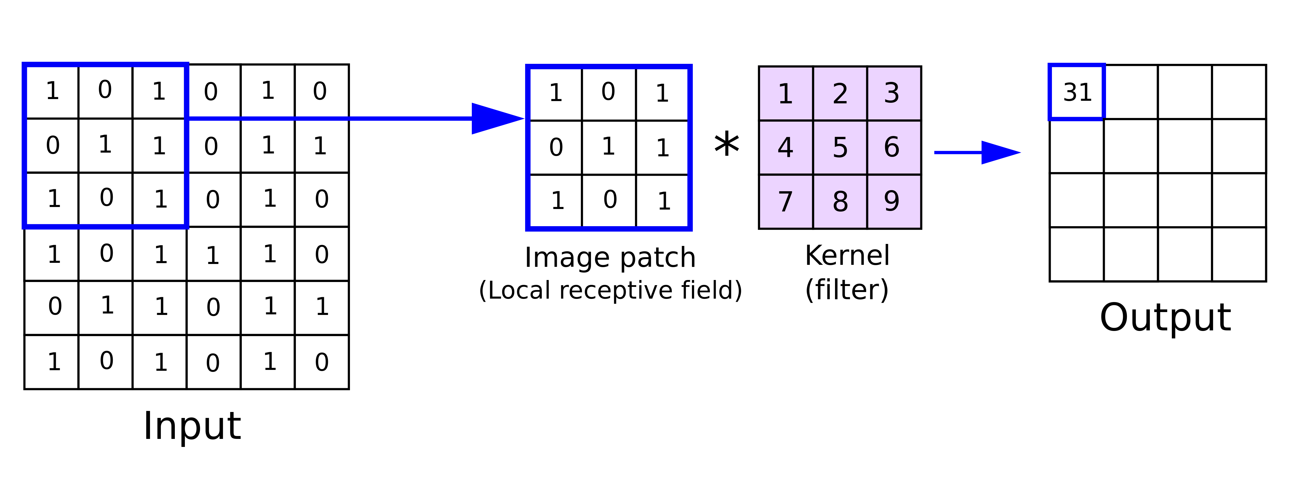
At the heart of CNNs lies a remarkably elegant operation called convolution. Imagine sliding a small window (a kernel or filter) across an image. At each position, we multiply the kernel values by the overlapping image pixels and sum the results to produce a single output value. Repeating this across all positions creates an output feature map.
Convolution operation. The kernel slides across the input, computing weighted sums at each position to produce a feature map.
Figure 1
Mathematically, for a single-channel input (grayscale image), 2D convolution is:
(I * K)_{i,j} = \sum_{m=0}^{L-1}\sum_{n=0}^{L-1} I_{i+m,j+n} \cdot K_{m,n}
where I is the input image, K is the kernel of size L \times L, and (i,j) specifies the output position.
What makes CNNs powerful is that these kernels are learnable parameters. During training, each kernel evolves to detect specific visual patterns like edges, textures, colors, or more complex features. The network discovers useful features automatically rather than relying on hand-crafted filters. Real-world images have multiple channels (RGB), and convolution extends naturally to 3D inputs using 3D kernels:
(I * K)_{i,j} = \sum_{c=1}^{C}\sum_{m=0}^{L-1}\sum_{n=0}^{L-1} I_{c,i+m,j+n} \cdot K_{c,m,n}
where C is the number of input channels. Each kernel processes all channels simultaneously, combining color information into a single output value.
Multi-channel convolution. Each kernel processes all input channels, producing one output feature map.
Figure 2
Interactive visualizations
Explore CNN operations interactively. The CNN Explainer shows how convolution, activation, and pooling work step-by-step. The Interactive Node-Link Visualization lets you see activations flow through a trained network.
Translation Equivariance: A Key Property
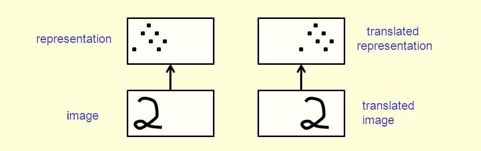
A crucial feature of convolutional layers is translation equivariance: if you shift the input, the output shifts by the same amount. When detecting a vertical edge, if the edge moves one pixel to the right in the input, the detected feature also moves one pixel to the right in the output. The detection operation cares only about relative patterns, not absolute position.
Translation equivariance. The same kernel detects the same feature regardless of position in the input.
Figure 3
This property allows CNNs to recognize objects anywhere in an image. A cat detector learned on centered cats will also detect cats in image corners, and the network doesn’t need to learn separate detectors for every possible position.
Parameter Sharing: Efficient Learning
Unlike fully connected networks where each weight is used once, convolutional layers reuse kernel weights across all spatial positions. A 3×3 kernel applied to a 224×224 RGB image uses just 27 parameters (3×3×3), not the millions required by a fully connected layer. This weight-sharing dramatically reduces parameter count while preserving spatial relationships, a key reason CNNs can process high-resolution images efficiently.
Receptive Field: Seeing More with Depth
The receptive field is the region of input pixels that influence each output pixel. In the first convolutional layer, a 3×3 kernel has a receptive field of 3×3 pixels. As we stack layers, the receptive field grows. Consider two 3×3 convolutional layers: each output pixel in the second layer depends on a 3×3 region in the first layer’s output, but each of those positions depends on a 3×3 region in the input, so the second layer’s receptive field is 5×5 in the original input.
Receptive field grows with network depth. Deeper layers see increasingly large regions of the input image.
Figure 4
Why does this matter? This hierarchical structure allows CNNs to detect increasingly complex, abstract features: early layers detect edges and simple patterns, middle layers combine these into textures and parts, and deep layers recognize complete objects and scenes.
Stride and Padding: Controlling Dimensions
Stride determines how many pixels we skip when sliding the kernel. With stride 1, we move one pixel at a time creating dense feature maps, while stride 2 skips every other position, effectively downsampling the output. For a 1D example with input [a,b,c,d,e,f] and kernel [1,2]:
Larger strides reduce computational cost and increase the receptive field but might miss fine details.
Stride controls how far the kernel moves at each step. Stride 2 produces half the spatial dimensions of stride 1.
Figure 5
Padding addresses information loss at borders. Without padding (called “valid” padding), the output shrinks after each convolution because the kernel can’t fully overlap with border pixels. Zero padding adds a border of zeros around the input, allowing the kernel to process edge pixels and control output dimensions.
Zero padding extends the input with zeros, preserving spatial dimensions and processing border pixels.
Figure 6
For a square input of size W with kernel size K, stride S, and padding P, the output dimension is:
O = \left\lfloor\frac{W - K + 2P}{S}\right\rfloor + 1
The interplay between stride and padding lets network designers control spatial dimensions and computational efficiency. Try the Convolution Visualizer to experiment with different stride and padding settings interactively.
Pooling Layers: Downsampling with Invariance
Pooling layers downsample feature maps, reducing spatial dimensions while preserving important information. Max pooling selects the maximum value in each local window:
P_{i,j} = \max_{m,n} F_{si+m,sj+n}
where F is the feature map, s is the stride (typically equal to the window size), and (m,n) range over the pooling window.
Max pooling creates local translation invariance: if an edge moves slightly within a pooling window, the maximum value remains unchanged, helping the network focus on whether a feature is present rather than its exact position. Pooling also reduces computational cost by decreasing spatial dimensions, and a common pattern is to double the number of channels while halving spatial dimensions, maintaining roughly constant computational load across layers. Some recent architectures replace pooling with strided convolutions, arguing that learnable downsampling might be more effective (Springenberg et al. 2015), though the choice involves trade-offs between parameter efficiency and flexibility.
Using Pre-Trained Models
Now that we understand CNN building blocks, let’s use them in practice. Training a CNN from scratch on ImageNet requires weeks of GPU time, but we can leverage pre-trained models trained by research labs with vast computational resources.
Loading Models from torchvision
PyTorch’s torchvision.models provides pre-trained implementations of major architectures:
import torchimport torchvision.models as modelsfrom torchvision import transformsfrom PIL import Imageimport requestsfrom io import BytesIO# Load a pre-trained ResNet-50 modelresnet50 = models.resnet50(weights='IMAGENET1K_V1')resnet50.eval() # Set to evaluation modeprint(f"Model type: {type(resnet50)}")print(f"Number of parameters: {sum(p.numel() for p in resnet50.parameters()):,}")
Model type: <class 'torchvision.models.resnet.ResNet'>
Number of parameters: 25,557,032
The model is trained on ImageNet with 1000 classes, and we can use it to classify images directly.
Image Classification Example
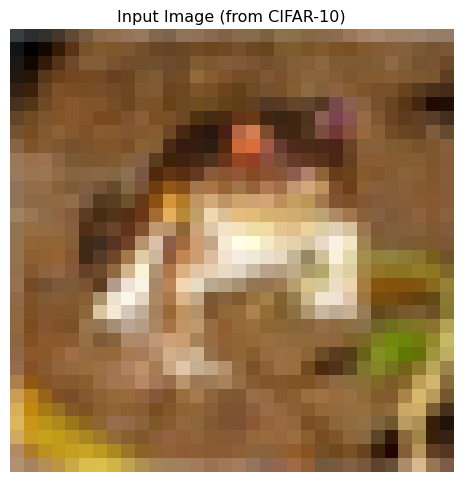
To use a pre-trained model, we must preprocess images the same way they were during training. ImageNet models expect images resized to 224×224 (or 299×299 for some models) with pixel values normalized to mean=[0.485, 0.456, 0.406] and std=[0.229, 0.224, 0.225].
The model correctly identifies the object with high confidence, demonstrating the power of pre-trained networks that have learned rich visual representations from ImageNet’s diverse images.
When to Use Which Architecture
Different architectures offer trade-offs between accuracy, speed, and memory. ResNet-50 provides excellent general-purpose performance with good accuracy and reasonable speed. EfficientNet is optimized for mobile and edge devices with the best accuracy-per-parameter ratio. VGG-16 has a simple, easy-to-understand architecture but is larger and slower than modern alternatives. MobileNet is designed for fast mobile inference at the cost of some accuracy. Vision Transformer (ViT) achieves state-of-the-art accuracy on large datasets but requires more data and compute. For most applications, start with ResNet-50 and optimize for speed or accuracy later if needed.
Transfer Learning: Adapting Pre-Trained Models
Pre-trained models learn general visual features from ImageNet’s 1000 categories, but what if you want to classify different objects? Transfer learning adapts these models to new tasks.
Why Transfer Learning Works
ImageNet-trained models learn a hierarchy of features: early layers detect edges, colors, and simple textures that are universal across tasks; middle layers detect patterns, parts, and compositions that are somewhat task-specific; late layers detect complete objects specific to ImageNet categories. The early and middle layers learn representations useful for many vision tasks, so we can reuse these features and only retrain the final layers for our specific problem.
Two Approaches: Feature Extraction vs. Fine-Tuning
Feature Extraction freezes all convolutional layers and trains only a new classifier head, running fast and working well with small datasets. Fine-Tuning initializes with pre-trained weights then trains the entire network (or parts of it) on your data, achieving better accuracy but requiring more data and computation.
Example: Fine-Tuning for Custom Classification
Let’s adapt ResNet-50 to classify 10 animal species:
import torch.nn as nnimport torch.optim as optim# Load pre-trained ResNet-50model = models.resnet50(weights='IMAGENET1K_V1')# Replace the final fully connected layer# Original: 2048 -> 1000 (ImageNet classes)# New: 2048 -> 10 (our custom classes)num_classes =10model.fc = nn.Linear(model.fc.in_features, num_classes)# Move model to GPU if availabledevice = torch.device("cuda"if torch.cuda.is_available() else"cpu")model = model.to(device)print(f"Modified final layer: {model.fc}")
Modified final layer: Linear(in_features=2048, out_features=10, bias=True)
For feature extraction, freeze early layers:
# Freeze all layers except the final classifierfor param in model.parameters(): param.requires_grad =False# Unfreeze the final layerfor param in model.fc.parameters(): param.requires_grad =True# Count trainable parameterstrainable_params =sum(p.numel() for p in model.parameters() if p.requires_grad)total_params =sum(p.numel() for p in model.parameters())print(f"Trainable parameters: {trainable_params:,} / {total_params:,}")
Trainable parameters: 20,490 / 23,528,522
Only 20,490 parameters (the final layer) are trainable, making training fast and preventing overfitting on small datasets.
Training Loop
Show training loop implementation
# Define loss and optimizercriterion = nn.CrossEntropyLoss()optimizer = optim.Adam(model.fc.parameters(), lr=0.001)# Training loop (pseudo-code, requires actual data)def train_epoch(model, dataloader, criterion, optimizer, device): model.train() running_loss =0.0 correct =0 total =0for inputs, labels in dataloader: inputs, labels = inputs.to(device), labels.to(device) optimizer.zero_grad() outputs = model(inputs) loss = criterion(outputs, labels) loss.backward() optimizer.step() running_loss += loss.item() _, predicted = torch.max(outputs, 1) total += labels.size(0) correct += (predicted == labels).sum().item() epoch_loss = running_loss /len(dataloader) epoch_acc = correct / totalreturn epoch_loss, epoch_acc# For fine-tuning instead of feature extraction:# 1. Unfreeze all or some layers# 2. Use a smaller learning rate (e.g., 1e-4 or 1e-5)# 3. Train for more epochs
Data Augmentation: Essential for Small Datasets
When training on limited data, augmentation is crucial: transform each image differently each epoch to artificially expand the training set.
Show training augmentation pipeline
# Training transforms with aggressive augmentationtrain_transform = transforms.Compose([ transforms.RandomResizedCrop(224), # Random crop and resize transforms.RandomHorizontalFlip(), # Flip with 50% probability transforms.ColorJitter( # Random brightness, contrast brightness=0.2, contrast=0.2, saturation=0.2 ), transforms.RandomRotation(15), # Rotate up to 15 degrees transforms.ToTensor(), transforms.Normalize( mean=[0.485, 0.456, 0.406], std=[0.229, 0.224, 0.225] ),])
Note that validation uses deterministic transforms (no randomness) for reproducible evaluation.
Best Practices for Transfer Learning
Start with feature extraction by training only the final layer first, which is fast and often achieves good results. If accuracy is insufficient, try fine-tuning by unfreezing earlier layers and training with a small learning rate (10× smaller than initial training). Use learning rate schedules to reduce the learning rate when validation loss plateaus. Monitor for overfitting using validation data, and apply more augmentation or stronger regularization (dropout, weight decay) if needed. Always match preprocessing to the pre-training dataset, using ImageNet statistics for most models.
Try it yourself
Practice transfer learning on your own image dataset. Collect 100-500 images per class (even phone camera photos work), then split into train/val/test sets (70/15/15). Start with ResNet-50 feature extraction and train for 10-20 epochs before evaluating on the test set. You’ll likely achieve 80-90%+ accuracy with just a few hundred images per class, demonstrating the power of pre-trained features.
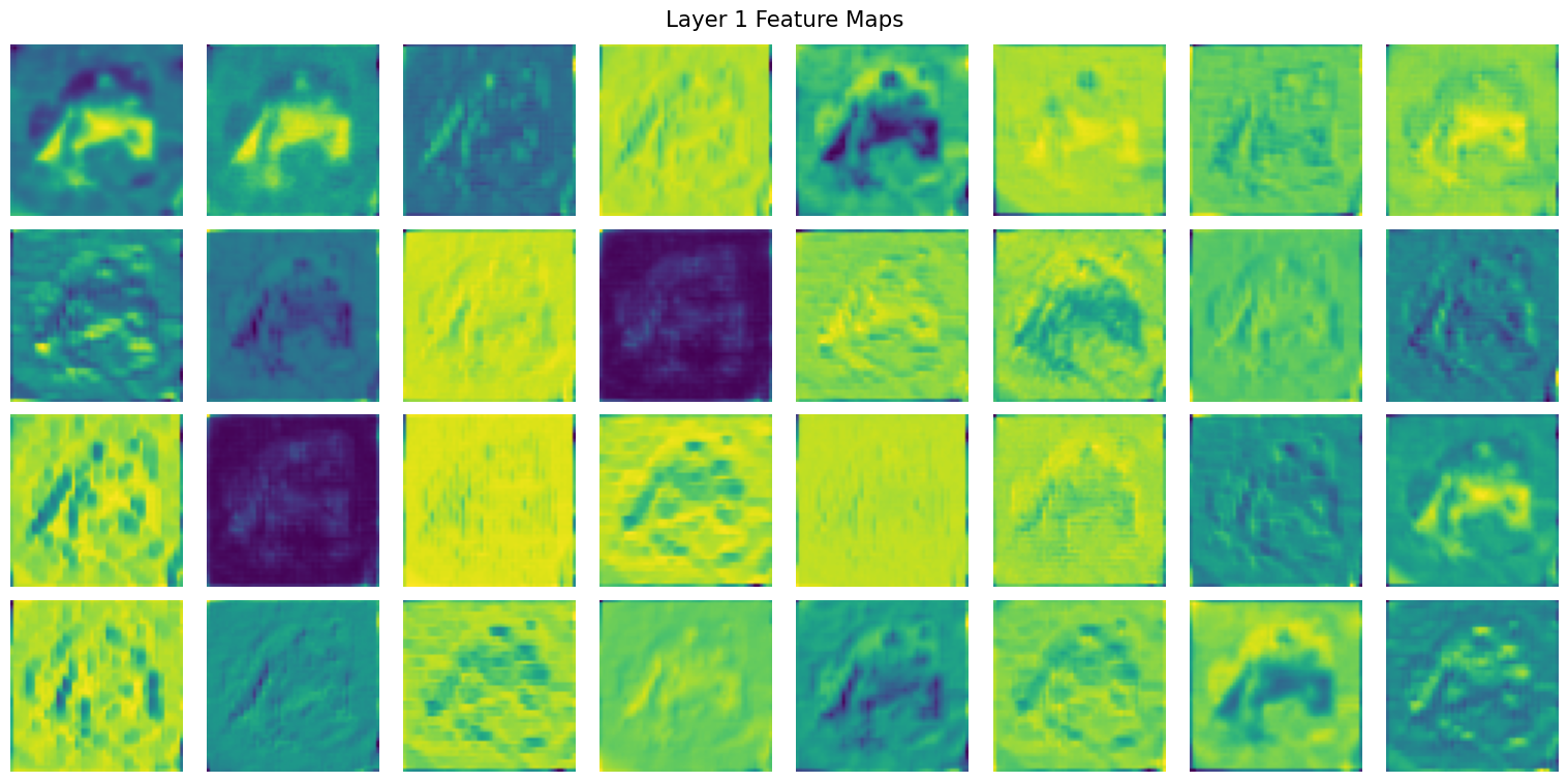
Visualizing What Networks Learn
What features do trained networks actually detect? Let’s peek inside a trained network to see:
Early layers show edge detection and simple patterns, while deeper layers show increasingly abstract features that are harder to interpret but encode high-level semantic information.
Summary
We explored the building blocks that make CNNs powerful: convolution operations with learnable kernels, translation equivariance for position-invariant recognition, parameter sharing for efficiency, growing receptive fields through depth, stride and padding for dimension control, and pooling for downsampling with invariance. We learned to use pre-trained models from torchvision and adapt them to custom tasks through transfer learning, either by feature extraction (training only the classifier) or fine-tuning (training the entire network with small learning rates). Data augmentation artificially expands small datasets to prevent overfitting. These practical skills let you load state-of-the-art models, adapt them to your data, and achieve strong results with limited computational resources.
References
Springenberg, Jost Tobias, Alexey Dosovitskiy, Thomas Brox, and Martin A. Riedmiller. 2015. “Striving for Simplicity: The All Convolutional Net.” In 3rd International Conference on Learning Representations, ICLR 2015, San Diego, CA, USA, May 7-9, 2015, Workshop Track Proceedings, edited by Yoshua Bengio and Yann LeCun. http://arxiv.org/abs/1412.6806.