Part 3: From Categories to Coordinates
This module introduces vector embeddings as the computational realization of structuralism.
You’ll learn:
- What vector embeddings are and how they dissolve artificial category boundaries.
- How word2vec learns meaning from context through the distributional hypothesis.
- The role of contrastive learning and negative sampling in carving semantic space.
- Why vector arithmetic captures relationships as geometric directions.
- How hyperbolic embeddings use geometry to capture hierarchy (metaphor) vs. association (metonymy).
- The counterintuitive insight that meaning emerges from exclusion (Apoha theory) and the notion of continuous representation.
- Practical consequences for understanding political ideology, semantic similarity, and beyond.
The Limits of Traditional Classification
Let’s talk about how traditional machine learning builds decision boundaries. You collect labeled data, extract features, and train a classifier to draw a line (or hyperplane) separating Class A from Class B. The output is binary: spam or not-spam, fraud or legitimate, cat or dog.
This approach works when categories are genuinely discrete. But what about political ideology? You might lean liberal on economic issues but conservative on others. Your position isn’t “left or right” but a point in a multidimensional space, and forcing it into a binary choice destroys information.
What about word meanings? Is “dog” more similar to “wolf” or “cat”? The answer is “it depends” on whether you care about biology (dogs and wolves share a genus) or domestication (dogs and cats are both pets). A classification system would force you to choose one dimension, while a continuous representation can capture both simultaneously.
Enter Vector Embeddings
Vector embeddings solve this by mapping each concept to coordinates in a high-dimensional continuous space. Instead of “this word belongs to category X”, you get “this word lives at position [0.23, -0.15, 0.87, ...] in 300-dimensional space”. Similarity becomes geometric distance, and relationships become directional vectors.
This is the mathematical realization of structuralism. Each word’s meaning is determined by its position relative to all other words. There are no hard boundaries, only neighborhoods of varying density.
How Word2Vec Works
Word2vec learns through a prediction task. Given a center word, predict the context words around it.
Specifically, the model of word2vec is given by
P(j \vert i) = \frac{\exp(u_i^\top v_j)}{\sum_{k \in \mathcal{V}} \exp(u_i^\top v_k)},
where u_i is the “in-vector” of center word i and v_j is the “out-vector” of context word j.
But here’s the problem. The denominator involves a sum over all words in the dictionary, which is not computable even for a moderate vocabulary size since we need to compute the probability of all words many times during training.
What’s the solution? Negative Sampling offers an elegant answer.
Instead of calculating probabilities over the entire dictionary, we play a simpler game. We give the model a pair of words and ask: “Is this a real context pair, or did I just randomly grab a word from the dictionary?”
The model tries to output 1 for real pairs and 0 for random (negative) pairs. Mathematically, we want to maximize this objective:
J(\theta) = \log \sigma(\mathbf{u}_w \cdot \mathbf{v}_c) + \sum_{i=1}^k \mathbb{E}_{v_n \sim P_n} [\log \sigma(-\mathbf{u}_w \cdot \mathbf{v}_{n})]
Here, \sigma is the sigmoid function that squashes values between 0 and 1. The first term encourages the model to put (v_c) close to (v_w). The second term encourages it to push (v_c) away from (v_n).
Why Does Negative Sampling Work?
We can prove that this seemingly ad-hoc contrastive training is actually doing the right thing. Let us write explicitly the sigmoid function:
p(y=1 \vert x) = \sigma(x) = \frac{1}{1 + \exp(-x)}
The probability that two words x=(i,j) are positive (i.e., y=1) relative to the probability that they are not (i.e., y=0) is given by:
\log \frac{p(y=1 \vert x)}{p(y=0 \vert x)} = x
Thus, the argument of the sigmoid function (i.e., x) represents the log-odds of the positive example, also called logits.
Now, let us make it clear that the negative samples are sampled from a probability distribution q. When observing a word pair x=(i,j), there are two possible events:
- y=1: The pair (i,j) is a real context pair, with probability p(i,j)
- y=0: The pair (i,j) is sampled by random chance, with probability q(i,j)
The probability that x comes from the positive class is given by:
p(y=1 \vert x) = \frac{p(i,j)}{p(i,j) + q(i,j)}
This is a sigmoid function, i.e.,
p(y=1 \vert x) = \frac{1}{1 + \exp\left(-\ln p(i,j) + \ln q(i,j)\right)}
with the logits given by
\ln p(i,j) - \ln q(i,j)
which word2vec expresses as the dot similarity of two vectors, i.e.,
u_i^\top v_j
Putting together we have
u_i^\top v_j = \ln p(i,j) - \ln q(j) \implies p(i,j) = \frac{q(i,j)\exp\left(u_i^\top v_j\right)}{\sum_{k \in \mathcal{V}} q(i,k)\exp\left(u_i^\top v_k\right)}
Therefore, negative sampling learns the word2vec model when sampling the negatives uniformly at random q(j) = \frac{1}{|\mathcal{V}|}.
In practice, the noise distribution q is not uniform but is (roughly) proportional to the frequency of the word j. Consequently, the learned model is not precisely the word2vec model but a variant with an inference bias. Yet, this bias is surprisingly useful in downstream tasks. See (Kojaku et al. 2021) and (Kojaku et al. 2023) for more details.
Word2Vec Implicitly Factorizes a Co-Occurrence Matrix
We have taken for granted that word2vec learns useful embeddings of words. But why are learned embeddings so useful despite being learned heuristically?
The previous section allows us to approach this theoretical question. It provides the analytical form of the similarity as:
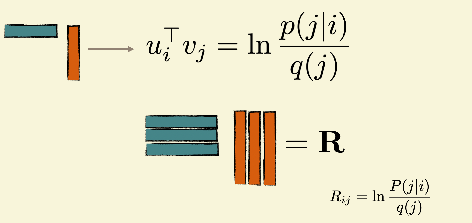
u_i^\top v_j = \ln p(i,j) - \ln q(j).
Notice that u_i, v_i have dimension d much smaller than the vocabulary size |\mathcal{V}|. On the other hand, the right hand side can have distinct values for each pair (i,j), forming a matrix with |\mathcal{V}|^2 entries.
From this perspective, word2vec is approximating this matrix by a product of two submatrices:
\mathbf{U} \cdot \mathbf{V}^\top = \mathbf{R},
where
\begin{align} \mathbf{R} &= \log p(i,j) - \log q(j) \\ \mathbf{U} &= \begin{bmatrix} u_1 \\ u_2 \\ \vdots \\ u_{|\mathcal{V}|} \end{bmatrix}, \mathbf{V} &= \begin{bmatrix} v_1 \\ v_2 \\ \vdots \\ v_{|\mathcal{V}|} \end{bmatrix} \end{align}
What does R_{ij} mean? The matrix entry R_{ij} has an information-theoretic meaning.
It is called the pointwise mutual information (PMI) between words i and j. In other words, the dot product of the vectors represents this information-theoretic quantity.
This is an interesting insight as it provides a clear interpretation of the learned embeddings. Furthermore, it also provides a clear analytical threshold as to when word2vec can capture groups and miss them. See (Kojaku et al. 2023) for more details.
A Universe of Contrast
This principle of pulling positive examples together while pushing negative ones apart grew into one of the most successful ideas in modern AI: Contrastive Learning.
Different tasks require different mathematical formulations of this “push-pull” dynamic.
Ranking & Triplet Loss
Used historically in systems like FaceNet for face recognition. The goal here is relative order.
We don’t care about the absolute coordinates, only that your face is closer to your own photos than to anyone else’s.
We define an anchor (a), a positive example (p), and a negative example (n). We want the distance d(a, p) to be smaller than d(a, n) by at least a margin m:
L = \max(0, d(a, p) - d(a, n) + m)
This forces a structured geometry where: d(a, p) + m < d(a, n). The model learns to “rank” the correct match higher than the incorrect one.
InfoNCE (SimCLR, CLIP)
This is the standard loss for modern self-supervised learning (like SimCLR or CLIP). Instead of comparing one positive against one negative, we play a game of “pick the correct partner from the lineup.”
Given a batch of N examples, the model must identify the single correct positive pair (i, j) against all other N-1 “negative” samples in the batch.
L_{i,j} = -\log \frac{\exp(\text{sim}(\mathbf{z}_i, \mathbf{z}_j) / \tau)}{\sum_{k=1}^{2N} \mathbb{1}_{[k \neq i]} \exp(\text{sim}(\mathbf{z}_i, \mathbf{z}_k) / \tau)}
It looks like a Softmax (specifically, categorical cross-entropy), but calculated only over the current batch rather than the full vocabulary. It forces the embedding to filter out specifically hard negatives from the current batch.
The Magic of Vector Arithmetic
Once you have vectors, you can do arithmetic on meaning. The famous example:
\vec{\text{King}} - \vec{\text{Man}} + \vec{\text{Woman}} \approx \vec{\text{Queen}}
Why does this work? Relationships are directions in space.
The vector from “Man” to “King” represents the relationship “royal-version-of”. When you apply that same direction to “Woman”, you arrive near “Queen”.
The arrows from countries to capitals are parallel. They point in roughly the same direction because they represent the same relationship.
This structure wasn’t programmed in. It emerged from observing how words co-occur in text.
The model discovered that “France” and “Paris” appear in similar contexts to how “Germany” and “Berlin” appear, and encoded this as geometric parallelism.
There are many such examples.
- Tshitoyan, V., Dagdelen, J., Weston, L., Dunn, A., Rong, Z., Kononova, O., … & Jain, A. (2019). Unsupervised word embeddings capture latent knowledge from materials science literature. Nature, 571(7763), 95-98.
- Peng, H., Ke, Q., Budak, C., Romero, D. M., & Ahn, Y. Y. (2021). Neural embeddings of scholarly periodicals reveal complex disciplinary organizations. Science Advances, 7(17), eabb9004.
- Kim, S., Ahn, Y. Y., & Park, J. (2024, May). Labor space: A unifying representation of the labor market via large language models. In Proceedings of the ACM Web Conference 2024 (pp. 2441-2451).
- Ke, Q. (2019). Identifying translational science through embeddings of controlled vocabularies. Journal of the American Medical Informatics Association, 26(6), 516-523.
Image Embeddings Also Exhibit Semantic Structure

This phenomenon isn’t limited to text. Generative models for images, such as VAEs (Variational Autoencoders) and GANs (Generative Adversarial Networks), learn a high-dimensional latent space where every point represents a possible image.
Just as with word embeddings, this space is semantically structured. Moving in a specific direction corresponds to a meaningful change in the image.
For example, we can calculate an attribute vector for “smiling” by taking the average position of all smiling faces and subtracting the average position of non-smiling faces:
\vec{v}_{\text{smile}} = \text{mean}(\text{smiling faces}) - \text{mean}(\text{neutral faces})
Adding this vector to the latent code of a new, neutral face will continuously transform it into a smiling one. This works for glasses, age, gender, and many other attributes.
The model doesn’t just memorize pixels. It learns the underlying factors of variation in the visual world. See White, T. (2016). Sampling generative networks. arXiv preprint arXiv:1609.04468..
Hyperbolic Embeddings
Shift your attention to a fundamental limitation in everything we’ve seen so far. Models like Word2Vec and GloVe are built on Metonymy (from the Greek meta “change” + onyma “name”), learning from the syntagmatic axis, the “next-to” relationship. “Crown” is embedded near “King” because they appear together in text context. They capture association.
But what about Metaphor? Metaphor relies on the paradigmatic axis, the “is-a” or “substitution” relationship. A “Lion” is implicitly like a “Tiger” not because they hang out together, but because they occupy the same structural slot in the hierarchy of life (they are both big cats).
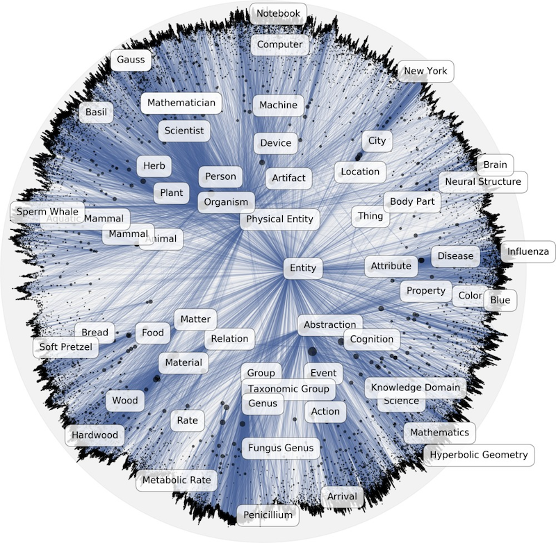
To capture this structural similarity, researchers turned to WordNet, a massive database explicitly constructed to map these “is-a” (hypernym) relationships. It is a map of taxonomies, effectively a giant tree of concepts.
When they tried to train standard Euclidean embeddings on WordNet, they hit a wall. Even with hundreds of dimensions, the models struggled to represent the deep, branching hierarchy without distorting the relationships. The problem wasn’t the data but the geometry itself.
Euclidean space is flat, but in a hierarchy (like a biological taxonomy or a corporate org chart), the number of nodes expands exponentially as you go deeper (Root \to Children \to Grandchildren). In flat space, the available volume only grows polynomially, so there simply isn’t enough “room” at the boundaries to fit this exponential growth. You end up crushing the leaf nodes together, losing the distinct structure.
To solve this, we need to exit flat space and enter Hyperbolic Space, often visualized as a Poincaré ball. In this non-Euclidean geometry, space itself expands exponentially as you move away from the center. Imagine a disk where, using a specific distance metric (Poincaré distance), the path to the edge is effectively infinite. Because the “room” available grows exactly as fast as the tree branches, you can fit an infinite tree structure within this finite disk by placing the root at the center, with the leaves fitting naturally near the boundary without crushing into each other.
This alignment of geometry and data is powerful. While Euclidean models might require 300 dimensions to separate concepts in WordNet, Poincaré embeddings can capture the same complex structure with high precision in as few as 5 dimensions.
When the geometry fits the data, when we model metaphor with a space designed for hierarchies, the representation becomes incredibly efficient.