import gensim.downloader as api
import numpy as np

# Load pre-trained Word2vec embeddings
model = api.load("word2vec-google-news-300")Word Bias
What you’ll learn in this module
This module explores how word embeddings capture and reinforce societal biases.
You’ll learn:
- How semantic axes reveal gender bias in occupations and concepts through geometric relationships.
- How to measure bias using cosine similarity and the SemAxis framework.
- The difference between direct bias (explicit gender associations) and indirect bias (gender encoded through proxy dimensions).
- Why understanding these biases matters for building fair AI systems.
Understanding Bias in Word Embeddings
Have you ever wondered what biases might be hiding in word embeddings? Word embeddings capture and reinforce societal biases from their training data through geometric relationships between word vectors, often reflecting stereotypes about gender, race, age, and other social factors.
SemAxis is a powerful tool to analyze gender bias in word embeddings by measuring word alignments along semantic axes. Using antonym pairs like “she-he” as poles, it quantifies gender associations in words on a scale from -1 to 1, where positive values indicate feminine associations while negative values indicate masculine associations. Let’s start with a simple example of analyzing gender bias in occupations.
def compute_bias(word, microframe, model):
    word_vector = model[word]
    numerator = np.dot(word_vector, microframe)
    denominator = np.linalg.norm(word_vector) * np.linalg.norm(microframe)
    return numerator / denominator


def analyze(word, pos_word, neg_word, model):
    if word not in model:
        return 0.0
    microframe = model[pos_word] - model[neg_word]
    bias = compute_bias(word, microframe, model)
    return bias
What’s happening in compute_bias? The function calculates the cosine similarity between a word vector and a semantic axis (microframe), where the numerator computes the dot product (projecting the word onto the axis) and the denominator normalizes by vector lengths to get a score between -1 and 1. Let’s use these occupations:
# Occupations from the paper
she_occupations = [
    "homemaker",
    "nurse",
    "receptionist",
    "librarian",
    "socialite",
    "hairdresser",
    "nanny",
    "bookkeeper",
    "stylist",
    "housekeeper",
]

he_occupations = [
    "maestro",
    "skipper",
    "protege",
    "philosopher",
    "captain",
    "architect",
    "financier",
    "warrior",
    "broadcaster",
    "magician",
    "boss",
]
We measure the gender bias in these occupations by measuring how they align with the “she-he” axis.
Code
print("Gender Bias in Occupations (she-he axis):")
print("\nShe-associated occupations:")
for occupation in she_occupations:
    bias = analyze(occupation, "she", "he", model)
    print(f"{occupation}: {bias:.3f}")

print("\nHe-associated occupations:")
for occupation in he_occupations:
    bias = analyze(occupation, "she", "he", model)
    print(f"{occupation}: {bias:.3f}")
Gender Bias in Occupations (she-he axis):
She-associated occupations:
homemaker: 0.360
nurse: 0.333
receptionist: 0.329
librarian: 0.300
socialite: 0.310
hairdresser: 0.307
nanny: 0.287
bookkeeper: 0.264
stylist: 0.252
housekeeper: 0.260
He-associated occupations:
maestro: -0.203
skipper: -0.177
protege: -0.148
philosopher: -0.155
captain: -0.130
architect: -0.151
financier: -0.145
warrior: -0.120
broadcaster: -0.124
magician: -0.110
boss: -0.090How do we interpret these scores? Positive scores indicate closer association to “she” (e.g., nurse, librarian), while negative scores indicate closer association to “he” (e.g., architect, captain), with magnitude showing the strength of association. Notice how occupations historically associated with women have strong positive scores while those associated with men have negative scores, confirming that the model has learned these gender stereotypes from the text data.
Stereotype Analogies
What happens when we look at word pairs? Since word embeddings capture semantic relationships from large text corpora, they inevitably encode societal biases and stereotypes. Let’s measure how different words align with the gender axis (she-he) to find pairs where one word shows strong feminine bias while its counterpart shows masculine bias, revealing ingrained stereotypes in language use.
# Stereotype analogies from the paper
stereotype_pairs = [
    ("sewing", "carpentry"),
    ("nurse", "surgeon"),
    ("softball", "baseball"),
    ("cosmetics", "pharmaceuticals"),
    ("vocalist", "guitarist"),
]
Code
print("\nAnalyzing Gender Stereotype Pairs:")
for word1, word2 in stereotype_pairs:
    bias1 = analyze(word1, "she", "he", model)
    bias2 = analyze(word2, "she", "he", model)
    print(f"\n{word1} vs {word2}")
    print(f"{word1}: {bias1:.3f}")
    print(f"{word2}: {bias2:.3f}")
Analyzing Gender Stereotype Pairs:

sewing vs carpentry
sewing: 0.302
carpentry: -0.028

nurse vs surgeon
nurse: 0.333
surgeon: -0.048

softball vs baseball
softball: 0.260
baseball: -0.066

cosmetics vs pharmaceuticals
cosmetics: 0.331
pharmaceuticals: -0.011

vocalist vs guitarist
vocalist: 0.140
guitarist: -0.041
The results show clear stereotypical alignments where sewing and nurse align with “she” while carpentry and surgeon align with “he”, mirroring the “man is to computer programmer as woman is to homemaker” analogy found in early word embedding research.
Indirect Bias: When Neutral Words Become Gendered
What about words that don’t explicitly reference gender? Indirect bias occurs when seemingly neutral words become associated with gender through their relationships with other words. For example, while “softball” and “football” are not inherently gendered terms, they may show gender associations due to how they’re used in language and society.
We can detect indirect bias by identifying word pairs that form a semantic axis (like softball-football), measuring how other words align with this axis, and examining if alignment correlates with gender bias. Let’s see how this works by measuring the gender bias of these words:
# Words associated with softball-football axis
softball_associations = [
    "pitcher",
    "bookkeeper",
    "receptionist",
    "nurse",
    "waitress"
]

football_associations = [
    "footballer",
    "businessman",
    "pundit",
    "maestro",
    "cleric"
]

# Calculate biases for all words
gender_biases = []
sports_biases = []
words = softball_associations + football_associations

for word in words:
    gender_bias = analyze(word, "she", "he", model)
    sports_bias = analyze(word, "softball", "football", model)
    gender_biases.append(gender_bias)
    sports_biases.append(sports_bias)
Let’s plot the results:
Code
# Analyze bias along both gender and sports axes
import matplotlib.pyplot as plt
import seaborn as sns
from adjustText import adjust_text

# Create scatter plot
fig, ax = plt.subplots(figsize=(6, 6))
sns.scatterplot(x=gender_biases, y=sports_biases, ax=ax)
ax.set_xlabel("Gender Bias (she-he)")
ax.set_ylabel("Sports Bias (softball-football)")
ax.set_title("Indirect Bias Analysis: Gender vs Sports")

# Add labels for each point
texts = []
for i, word in enumerate(words):
    texts.append(ax.text(gender_biases[i], sports_biases[i], word, fontsize=12))

adjust_text(texts, arrowprops=dict(arrowstyle='-', color='gray', lw=0.5))

ax.grid(True, alpha=0.3)
plt.show()
sns.despine()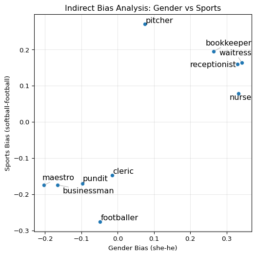
<Figure size 672x480 with 0 Axes>The plot reveals a correlation where words associated with “softball” (y-axis greater than 0) also tend to be associated with “she” (x-axis greater than 0), while “football” terms align with “he”. This suggests that even if we remove explicit gender words, the structure of the space still encodes gender through these proxy dimensions.
The Impact and Path Forward
Word embeddings, while powerful, inevitably capture and reflect societal biases present in the large text corpora they are trained on. We observed both direct bias (where occupations or attributes align strongly with specific gender pronouns) and indirect bias (where seemingly neutral concepts become gendered through their associations with other words). This analysis highlights the importance of understanding and mitigating these biases to prevent the perpetuation of stereotypes in AI systems and ensure fairness in applications like search, recommendation, and hiring.