# Define the vertical edge detection kernel
K_v = np.array([[-1, -1, -1],
                [0, 0, 0],
                [1, 1, 1]])

# Apply convolution to detect edges
edges = convolve2d(img_gray, K_v, mode='same', boundary='symm')Part 2: The Deep Learning Revolution
What you’ll learn in this module
This section traces the paradigm shift in computer vision from hand-crafted features to learned representations.
You’ll learn:
- How researchers designed edge detectors and frequency transforms by hand before deep learning.
- What LeNet contributed by pioneering automated feature learning in the 1990s.
- Why AlexNet’s 2012 breakthrough demonstrated that deep learning works at scale.
- The key innovations (ReLU, Dropout, GPU acceleration, data augmentation) that made AlexNet successful.
The Old Way: Engineering Features by Hand
Before 2012, computer vision meant one thing: carefully designing features by hand. Experts would analyze problems and craft mathematical operations to extract useful information like edge detection, texture analysis, and object boundaries. Let’s explore how this worked by examining edge detection, one of the fundamental problems in image processing.
Detecting Edges Through Brightness Changes
What makes an edge visible to human eyes? Sudden changes in brightness, appearing when neighboring pixels have significantly different intensity values. Recall from Part 1 the small 6×6 grayscale image with a bright vertical line in the third column (values of 80) surrounded by dark pixels (values of 10).
We can approximate the horizontal derivative by subtracting the right neighbor from the left neighbor at each position. For the central pixel, this looks like:
\nabla Z_{22} = Z_{2,1} - Z_{2,3}
Applied to the entire image, we get large values where brightness changes suddenly (the edge) and near-zero values elsewhere. This simple operation reveals structure.
Convolution: A General Pattern Matching Operation
The derivative calculation we just performed is a special case of a more general operation called convolution. The idea is elegant: define a small matrix of weights called a kernel or filter, then slide it across the image, computing weighted sums at each position.
For a 3×3 kernel K applied to a local patch Z:
\text{output}_{i,j} = \sum_{m=-1}^{1} \sum_{n=-1}^{1} K_{m,n} \cdot Z_{i+m, j+n}
The Prewitt operator provides kernels specifically designed for edge detection:
K_h = \begin{bmatrix} -1 & 0 & 1 \\ -1 & 0 & 1 \\ -1 & 0 & 1 \end{bmatrix} \quad\text{and}\quad K_v = \begin{bmatrix} -1 & -1 & -1 \\ 0 & 0 & 0 \\ 1 & 1 & 1 \end{bmatrix}
The horizontal kernel K_h detects vertical edges, while the vertical kernel K_v detects horizontal edges. Each kernel responds strongly when the image patch matches its pattern.
Show visualization code
fig, axes = plt.subplots(1, 2, figsize=(12, 5))
axes[0].imshow(img_gray, cmap='gray')
axes[0].set_title("Original Grayscale Image")
axes[0].axis("off")

axes[1].imshow(edges, cmap='gray')
axes[1].set_title("Vertical Edge Detection (Prewitt Filter)")
axes[1].axis("off")

plt.tight_layout()
plt.show()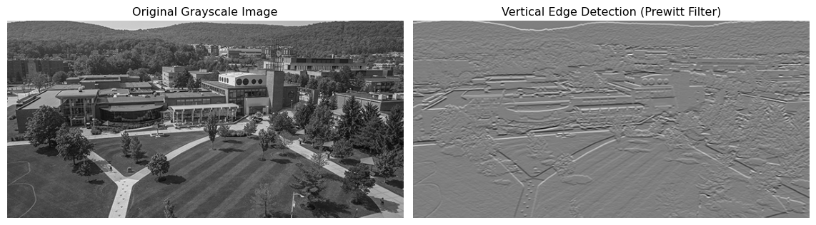
Notice how the filter highlights horizontal boundaries where brightness changes rapidly in the vertical direction. An excellent interactive demo of various image kernels can be found at Setosa Image Kernels.
Thinking in Frequencies: The Fourier Transform
Shift your attention from the spatial domain to the frequency domain. The Fourier transform represents images as combinations of sinusoidal patterns at different frequencies. For a discrete signal x[n] of length N, the Discrete Fourier Transform is:
\mathcal{F}(x)[k] = \sum_{n=0}^{N-1} x[n] \cdot e^{-2\pi i \frac{nk}{N}}
Using Euler’s formula e^{ix} = \cos(x) + i\sin(x), we can rewrite this as:
\mathcal{F}(x)[k] = \sum_{n=0}^{N-1} x[n]\Big[\cos(2\pi \tfrac{nk}{N}) - i\sin(2\pi \tfrac{nk}{N})\Big]
The Fourier transform decomposes a signal into its frequency components, where low frequencies correspond to smooth, slowly varying regions and high frequencies correspond to sharp edges and fine details. The convolution theorem reveals a beautiful connection: convolution in the spatial domain is equivalent to multiplication in the frequency domain:
X * K \quad\longleftrightarrow\quad \mathcal{F}(X) \cdot \mathcal{F}(K)
This means we can perform convolution by: 1. Taking the Fourier transform of both the image and the kernel 2. Multiplying them element-wise in the frequency domain 3. Taking the inverse Fourier transform to get back to the spatial domain
For large images, this approach can be computationally faster than direct convolution. For a beautiful visual explanation of the Fourier Transform, see 3Blue1Brown’s video.
The Fundamental Limitation
Here’s the problem with hand-crafted features: experts had to design every single one. Want to detect corners? Design a corner detector. Need to recognize textures? Craft texture descriptors. Each feature required mathematical sophistication and domain expertise, creating a feature engineering bottleneck that limited what computer vision could achieve. This approach worked for simple, well-defined tasks but scaled poorly to complex problems like recognizing thousands of object categories.
The First Breakthrough: LeNet
Have you ever wondered if there’s a better way? Yann LeCun posed a radical question in the late 1980s: what if networks could learn features automatically from raw pixels? Instead of hand-designing edge detectors, let the network discover useful patterns through training. This vision led to LeNet, a pioneering convolutional architecture that demonstrated automated feature learning on handwritten digit recognition (LeCun et al. 1989, 1998).
Architecture: Hierarchical Feature Learning
LeNet introduced a pattern that remains fundamental to modern CNNs:
- Convolutional layers apply learnable filters (not hand-designed) to extract local patterns
- Pooling layers downsample feature maps, creating spatial invariance
- Stacking multiple layers builds increasingly abstract representations
- Fully connected layers at the end combine features for classification
The key innovation was making the convolutional filters learnable parameters. During training, backpropagation adjusts filter weights to extract features useful for the task. The network discovers edge detectors, corner detectors, and more complex patterns automatically.
LeNet-5, the most influential version, processed 32×32 grayscale images through this architecture:
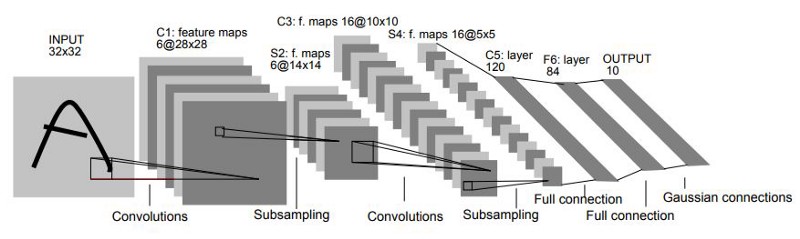
Let’s understand each component:
C1: First Convolutional Layer Takes the input image and applies learnable 5×5 filters. These filters start random but evolve during training to detect basic patterns like edges at various orientations.
S2: Subsampling (Pooling) Reduces spatial dimensions through average pooling with 2×2 windows. This creates local translation invariance—small shifts in feature positions don’t change the output significantly.
C3: Second Convolutional Layer Combines features from the previous layer to build more complex patterns. LeNet-5 used sparse connectivity here (not every feature map connects to every previous map), reducing parameters while encouraging diverse features.
S4: Second Subsampling Further reduces spatial dimensions, allowing the network to focus on increasingly abstract representations.
Fully Connected Layers Flatten the spatial feature maps into a vector and make the final classification decision across 10 digit classes.
Yann LeCun’s work on applying backpropagation to convolutional architectures in the 1980s was met with skepticism. But LeNet’s success on real-world tasks like automated check reading at banks helped spark wider interest in neural networks.
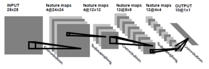
LeNet Architecture in Code
Here’s a simplified LeNet-1 implementation showing the core architecture:
Show LeNet-1 implementation
import torch
import torch.nn as nn

class LeNet1(nn.Module):
    """Simplified LeNet-1 architecture."""

    def __init__(self):
        super().__init__()
        self.conv1 = nn.Conv2d(1, 4, kernel_size=5)
        self.pool = nn.AvgPool2d(kernel_size=2, stride=2)
        self.conv2 = nn.Conv2d(4, 12, kernel_size=5)
        self.fc = nn.Linear(12 * 4 * 4, 10)

    def forward(self, x):
        x = torch.tanh(self.conv1(x))
        x = self.pool(x)
        x = torch.tanh(self.conv2(x))
        x = self.pool(x)
        x = x.view(-1, 12 * 4 * 4)
        x = self.fc(x)
        return x

model = LeNet1()
print(f"Total parameters: {sum(p.numel() for p in model.parameters()):,}")
Total parameters: 3,246This simple architecture achieves high accuracy on MNIST, demonstrating the power of learned features. The convolutional filters automatically discover edge detectors and pattern recognizers through training. We’ll explore how to train models like this in detail in Part 3.
Why LeNet Mattered
LeNet proved a crucial concept: networks can learn better features than human experts can design. This automated feature learning was revolutionary, but LeNet’s impact remained limited. It worked well on simple tasks like digit recognition but struggled with complex, large-scale problems because the computational constraints of the 1990s prevented training deeper networks (no GPU acceleration, small datasets, primitive training techniques). For nearly two decades, hand-crafted features like SIFT (Scale-Invariant Feature Transform) and HOG (Histogram of Oriented Gradients) powered most practical systems, while neural networks remained research curiosities. Then came 2012.
The Revolution: AlexNet
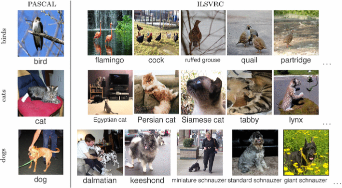
The ImageNet Large Scale Visual Recognition Challenge (ILSVRC) posed a formidable test: classify images into 1000 categories using a training set of 1.2 million images. This scale dwarfed anything LeNet had tackled, and the best systems in 2011 achieved around 25% top-5 error using carefully engineered features and traditional machine learning methods.
In 2012, Alex Krizhevsky, Ilya Sutskever, and Geoffrey Hinton submitted a deep convolutional network that reduced top-5 error to 16.4%. This more than 10 percentage point improvement shocked the community (Krizhevsky, Sutskever, and Hinton 2012).
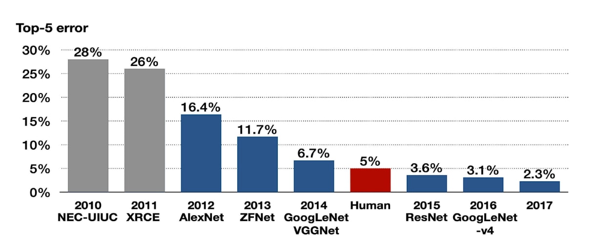
AlexNet didn’t just win. It demonstrated that deep learning could work at scale, igniting the revolution that transformed computer vision, speech recognition, natural language processing, and countless other domains.
Key Innovation 1: ReLU Activation
Why did deep networks fail before AlexNet? Deep networks suffer from the vanishing gradient problem, where gradients shrink as they flow backward through layers. Traditional activations like sigmoid \sigma(x) = \frac{1}{1 + e^{-x}} saturate for large positive or negative inputs, driving gradients toward zero and making early layers nearly impossible to train. AlexNet popularized the Rectified Linear Unit (ReLU) (Nair and Hinton 2010):
\text{ReLU}(x) = \max(0, x)

ReLU offers critical advantages: no vanishing gradient for positive inputs (gradient is exactly 1), computationally cheap (requires only a comparison to zero), and sparse activation where many neurons output zero for efficient representations. The drawback is that neurons can “die” if they always receive negative inputs, never activating again. Variants like Leaky ReLU introduce a small slope for negative inputs to mitigate this:
\text{Leaky ReLU}(x) = \begin{cases} x & \text{if } x > 0 \\ \alpha x & \text{if } x \leq 0 \end{cases}
where \alpha is typically 0.01.
Key Innovation 2: Dropout Regularization
Deep networks with millions of parameters easily overfit training data. AlexNet introduced Dropout as a powerful regularization technique (Srivastava et al. 2014).
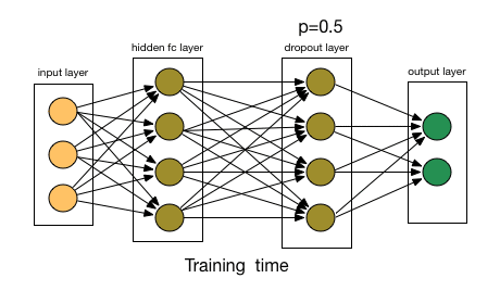
During training, Dropout randomly sets neuron outputs to zero with probability p (typically 0.5), preventing the network from relying too heavily on any single neuron. The effect is like training an ensemble of networks that share weights. At inference time, all neurons are active but their outputs are scaled by (1-p) to maintain expected values (modern implementations often use inverse dropout, scaling during training instead).
Key Innovation 3: GPU Acceleration
AlexNet demonstrated that deep learning needed massive computational power. The network was trained on two GPUs with 3GB memory each, splitting the computation to handle the large parameter count. This wasn’t just an implementation detail—it showed that deep learning required specialized hardware and helped catalyze the GPU computing revolution that continues today, with modern networks training on dozens or hundreds of GPUs.
Key Innovation 4: Data Augmentation
To combat overfitting with limited training data, AlexNet applied aggressive data augmentation: random crops of 224×224 patches from 256×256 images, horizontal flips, and color and lighting perturbations through PCA-based color jittering. These transformations artificially expanded the training set, teaching the network to recognize objects regardless of position, orientation, or lighting conditions.
The Architecture
AlexNet consists of five convolutional layers followed by three fully connected layers:
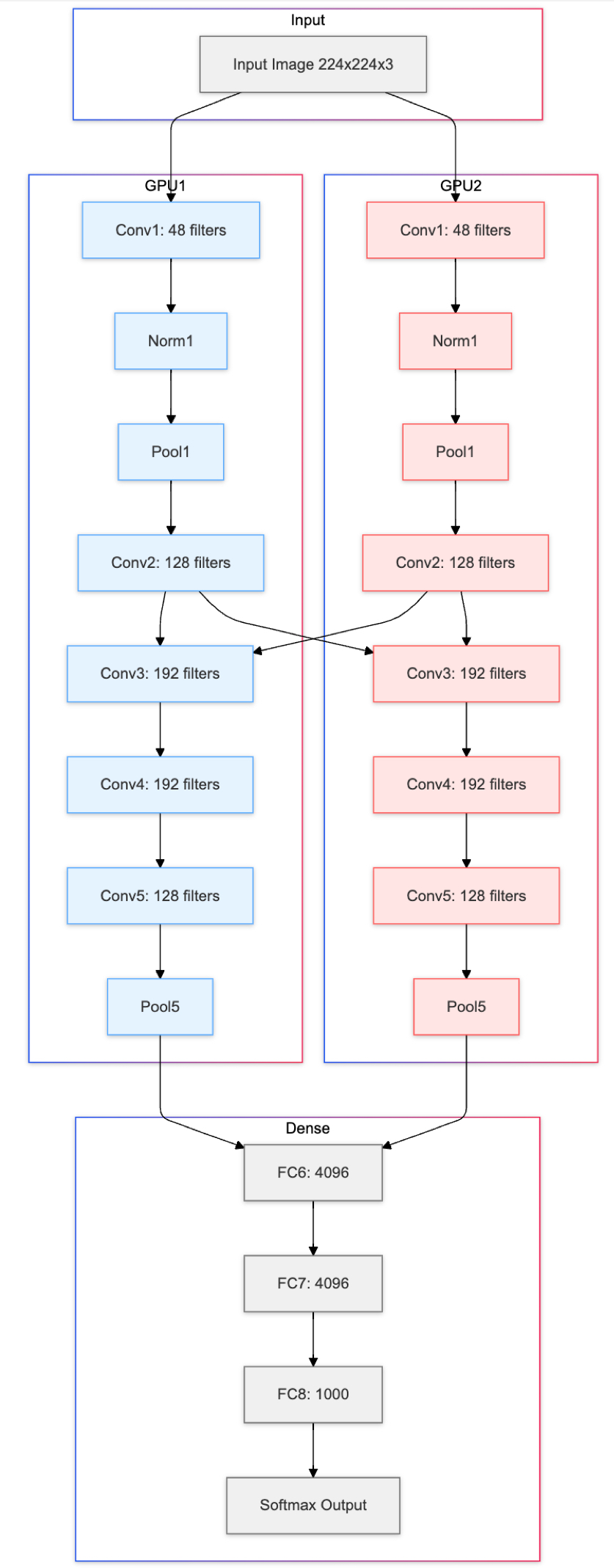
The architecture processes a 224×224 RGB image through the following layers. Conv1 applies 96 filters of 11×11 with stride 4, followed by ReLU and max pooling (3×3, stride 2), then Conv2 uses 256 filters of 5×5 with ReLU and max pooling. Conv3, Conv4, and Conv5 apply 384, 384, and 256 filters respectively using 3×3 kernels, with the final convolutional layer followed by max pooling. Three fully connected layers complete the network: FC6 and FC7 each contain 4096 neurons with ReLU and Dropout, while FC8 outputs 1000 class scores through Softmax.
The network has approximately 60 million parameters. The first convolutional layer uses large 11×11 filters with stride 4 to rapidly reduce spatial dimensions, while later layers use smaller 3×3 filters to refine features. AlexNet also used Local Response Normalization (LRN) to normalize activations across adjacent channels, though this technique is less common in modern architectures which typically use batch normalization instead.
Using Pre-Trained AlexNet
Rather than implementing AlexNet from scratch, we can leverage pre-trained models. PyTorch provides AlexNet trained on ImageNet, ready to use:
import torch
import torchvision.models as models

# Load pre-trained AlexNet
alexnet = models.alexnet(weights='IMAGENET1K_V1')
alexnet.eval()

print(f"Total parameters: {sum(p.numel() for p in alexnet.parameters()):,}")
Total parameters: 61,100,840This pre-trained model has learned rich visual representations from ImageNet’s 1.2 million images. In Part 3, we’ll explore how to use and adapt these pre-trained models for practical applications.
Why AlexNet Was a Paradigm Shift
AlexNet proved several critical points that transformed the field: depth matters (deeper networks learn more powerful representations), data scale matters (large datasets like ImageNet’s 1.2M images enable better learning), compute matters (GPUs make training deep networks practical), and learned features win (automated feature learning beats hand-crafted features). Before AlexNet, these points were debated; after AlexNet, they became accepted wisdom. Within months, researchers worldwide abandoned hand-crafted features, every computer vision competition became a deep learning competition, and companies invested billions in GPU infrastructure.
From Revolution to Practice
AlexNet demonstrated that deep learning works at scale. But how do we actually use these powerful models in practice, understand what’s happening inside these black boxes, and build networks with hundreds of layers? These questions lead us to the practical skills and advanced architectures we’ll explore in the remaining sections.
Summary
We traced computer vision’s evolution from hand-crafted features to learned representations. Traditional approaches required experts to design edge detectors, Fourier transforms, and pattern recognizers for each task, creating a feature engineering bottleneck that limited the field’s potential. LeNet pioneered automated feature learning in the 1990s, showing that networks could discover useful patterns through training, but computational limits constrained its impact.
AlexNet’s 2012 breakthrough on ImageNet changed everything with key innovations: ReLU activation (solving vanishing gradients), Dropout (preventing overfitting), and GPU acceleration (enabling large-scale training). The 10+ percentage point improvement shocked the computer vision community and sparked the deep learning revolution. This paradigm shift transformed how we approach machine perception—networks now learn features automatically from data, outperforming carefully engineered alternatives.
References
Krizhevsky, Alex, Ilya Sutskever, and Geoffrey E Hinton. 2012. “ImageNet Classification with Deep Convolutional Neural Networks.” In Advances in Neural Information Processing Systems, edited by F. Pereira, C. J. Burges, L. Bottou, and K. Q. Weinberger. Vol. 25. Curran Associates, Inc. https://proceedings.neurips.cc/paper_files/paper/2012/file/c399862d3b9d6b76c8436e924a68c45b-Paper.pdf.
LeCun, Yann, Bernhard E. Boser, John S. Denker, Donnie Henderson, Richard E. Howard, Wayne E. Hubbard, and Lawrence D. Jackel. 1989. “Backpropagation Applied to Handwritten Zip Code Recognition.” Neural Computation 1: 541–51. https://api.semanticscholar.org/CorpusID:41312633.
LeCun, Yann, Léon Bottou, Yoshua Bengio, and Patrick Haffner. 1998. “Gradient-Based Learning Applied to Document Recognition.” Proceedings of the IEEE 86 (11): 2278–2324.
Nair, Vinod, and Geoffrey E. Hinton. 2010. “Rectified Linear Units Improve Restricted Boltzmann Machines.” In Proceedings of the 27th International Conference on International Conference on Machine Learning, 807–14. ICML’10. Madison, WI, USA: Omnipress.
Srivastava, Nitish, Geoffrey Hinton, Alex Krizhevsky, Ilya Sutskever, and Ruslan Salakhutdinov. 2014. “Dropout: A Simple Way to Prevent Neural Networks from Overfitting.” The Journal of Machine Learning Research 15 (1): 1929–58.