Tokenization: Unboxing How LLMs Read Text

What you’ll learn in this module

This module introduces tokenization, the subword compression strategy that powers modern language models.

You’ll learn:

• What tokens are and why LLMs use subwords instead of whole words.
• How subword tokenization reduces memory costs while enabling rare word handling.
• The complete pipeline from raw text to token IDs to embeddings.
• Why compression artifacts cause strange LLM behaviors like failing at character counting.

Why Not Just Words?

Have you ever wondered how an LLM reads text? You might assume it reads word by word, treating each word as an atomic unit. This assumption is wrong.

The model operates on tokens, which are subword chunks. These could be full words like “the”, word parts like “ingham”, or single characters like “B”. This choice isn’t arbitrary. It’s a geometric compression strategy.

Why compress? If we used whole words, the vocabulary would balloon to millions of entries. Each entry requires a row in the embedding matrix, so memory scales linearly with vocabulary size. A 1-million-word vocabulary with 2048-dimensional embeddings would require over 8GB just for the lookup table.

Subword tokenization collapses this problem by focusing on frequently occurring fragments. With roughly 50,000 subwords, the model reconstructs both common words (stored as single tokens) and rare words (assembled from parts). The system trades a small increase in sequence length for massive reductions in memory and computational overhead.

This compression explains a strange quirk. Why do LLMs sometimes fail at seemingly trivial tasks like counting letters? The word “strawberry” might tokenize as [“straw”, “berry”], meaning the model never sees individual “r” characters as separate units. It’s not stupidity. It’s compression artifacts.

How Tokenization Works in Practice

Let’s unbox an actual tokenizer from Hugging Face and trace the pipeline from raw text to embeddings. We’ll use Phi-1.5, a compact model from Microsoft.

For tokenization experiments, we only need the tokenizer itself, not the full multi-gigabyte model.

from transformers import AutoTokenizer
import os

model_name = "microsoft/phi-1.5"
tokenizer = AutoTokenizer.from_pretrained(model_name)

Let’s inspect the tokenizer’s constraints.

print(f"Vocabulary size: {tokenizer.vocab_size:,} tokens")
print(f"Max sequence length: {tokenizer.model_max_length} tokens")

Vocabulary size: 50,257 tokens
Max sequence length: 2048 tokens

This tokenizer knows 50,257 unique tokens and enforces a maximum sequence length of 2048 tokens. If your input exceeds this limit, the model will truncate or reject it. This is a hard boundary imposed by the positional encoding system, not a soft guideline.

From Text to Tokens

Tokenization splits text into the subword fragments the model actually processes. Watch what happens when we tokenize a university name.

text = "Binghamton University."

tokens = tokenizer.tokenize(text)

print(f"Tokens: {tokens}")

Tokens: ['B', 'ingham', 'ton', 'ĠUniversity', '.']

The rare word “Binghamton” fractures into [‘B’, ‘ingham’, ‘ton’]. The common word “University” survives intact (with a leading space marker). The tokenizer learned these splits from frequency statistics during training. High-frequency words get dedicated tokens. Rare words get decomposed into reusable parts.

What’s that Ġ character? The Ġ character (U+0120) is a GPT-style tokenizer convention for encoding spaces. When you see ĠUniversity, it means “University” preceded by a space. This preserves word boundaries while allowing subword splits.

Let’s test a few more examples to see the pattern.

texts = [
    "Bearcats",
    "New York",
]

print("Word tokenization examples:\n")
for text in texts:
    tokens = tokenizer.tokenize(text)
    print(f"{text:10s} → {tokens}")

Word tokenization examples:

Bearcats   → ['Bear', 'cats']
New York   → ['New', 'ĠYork']

“Bearcats” splits because it’s domain-specific jargon. “New York” remains whole because it’s common. The tokenizer’s behavior directly reflects its training corpus.

Check out OpenAI’s tokenizer to see how different models slice the same text differently.

From Tokens to Token IDs

Tokens are still strings. The model needs integers. Each token maps to a unique ID in the vocabulary dictionary.

text = "Binghamton University"

# Get token IDs
token_ids = tokenizer.encode(text, add_special_tokens=False)
tokens = tokenizer.tokenize(text)

print("Token → Token ID mapping:\n")
for token, token_id in zip(tokens, token_ids):
    print(f"{token:10s} → {token_id:6d}")

Token → Token ID mapping:

B          →     33
ingham     →  25875
ton        →   1122
ĠUniversity →   2059

Each token receives a unique integer ID. The vocabulary is a dictionary mapping token strings to integer IDs. Let’s peek inside.

# Get the full vocabulary
vocab = tokenizer.get_vocab()

# Sample some tokens
sample_tokens = list(vocab.items())[:5]
for token, id in sample_tokens:
    print(f"  {id:6d}: '{token}'")

   31818: 'Ġinconvenience'
   39472: 'Ġunknow'
   31083: 'Ġconcluding'
   35540: 'Ġ;)'
    5506: 'ĠAnn'

Most LLMs reserve special tokens for sequence boundaries or control signals. Phi-1.5 uses <|endoftext|> as a separator during training. Let’s verify.

token_id = [50256]
token = tokenizer.convert_ids_to_tokens(token_id)[0]
print(f"Token ID: {token_id} → Token: {token}")

Token ID: [50256] → Token: <|endoftext|>

Token ID 50256 is Phi-specific. Other models use different conventions (BERT uses [SEP] and [CLS]). Always check your tokenizer’s special tokens before preprocessing data.

From Token IDs to Embeddings

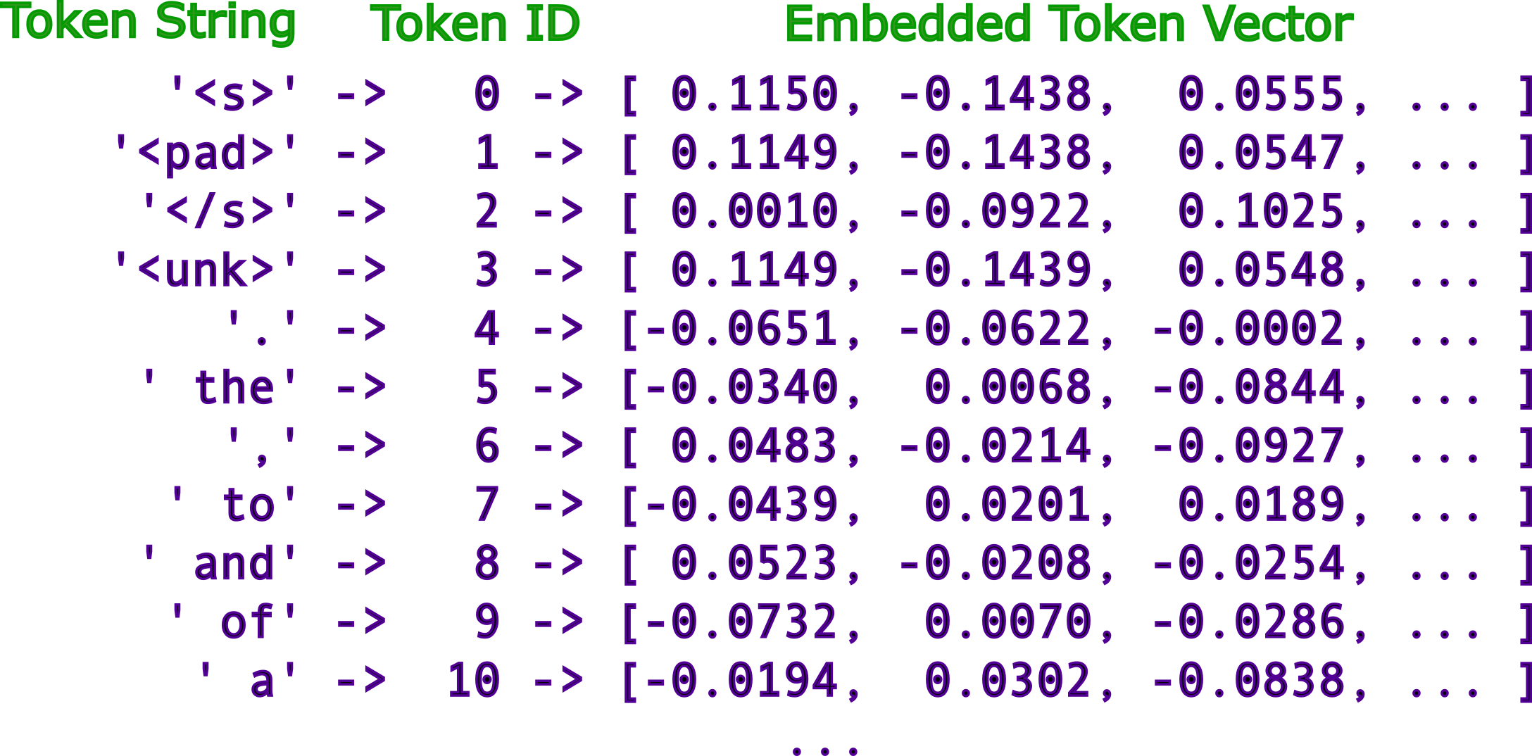
Now we need the full model to access the embedding layer, the matrix that converts token IDs into dense vectors.

from transformers import AutoModelForCausalLM
import torch

# Load the model
model = AutoModelForCausalLM.from_pretrained(model_name)

# Retrieve the embedding layer
embedding_layer = model.model.embed_tokens

The embedding layer is a simple lookup table. It’s a 51,200 × 2,048 matrix where each row is the embedding for a token in the vocabulary. Let’s examine the first few entries.

print(embedding_layer.weight[:5, :10])

tensor([[ 0.0097, -0.0155,  0.0603,  0.0326, -0.0108, -0.0271, -0.0273,  0.0178,
         -0.0242,  0.0100],
        [ 0.0243,  0.0543,  0.0178, -0.0679, -0.0130,  0.0265, -0.0423, -0.0287,
         -0.0051, -0.0179],
        [-0.0416,  0.0370, -0.0160, -0.0254, -0.0371, -0.0208, -0.0023,  0.0647,
          0.0468,  0.0013],
        [-0.0051, -0.0044,  0.0248, -0.0489,  0.0399,  0.0005, -0.0070,  0.0148,
          0.0030,  0.0070],
        [ 0.0289,  0.0362, -0.0027, -0.0775, -0.0136, -0.0203, -0.0566, -0.0558,
          0.0269, -0.0067]], grad_fn=<SliceBackward0>)

These numbers are learned parameters, optimized during training to capture semantic relationships. Token IDs are discrete symbols. Embeddings are continuous coordinates in a 2048-dimensional space. This is what the transformer layers operate on.

The Full Pipeline

You’ve now traced the complete pipeline. Raw text fractures into subword tokens, tokens map to integer IDs, and IDs retrieve vector embeddings from a learned matrix. This tokenization step is foundational. Without it, the model cannot begin processing language.

What comes next? The transformer layers come next, using attention mechanisms to extract patterns from these embeddings.

Remember three key constraints. First, LLMs operate on subwords, not words, because vocabulary size is a memory bottleneck. Second, tokenization is learned from data, not hand-designed, so different models split text differently. Third, compression has side effects. Tasks like character counting fail because the model never sees individual characters as atomic units.

With this machinery exposed, we’re ready to examine the transformer itself. It’s the architecture that processes these embeddings and enables LLMs to predict the next token.

---

Next: Transformers: The Architecture Behind the Magic