Part 4: The Innovation Timeline
This module traces CNN evolution through successive innovations that solved specific architectural challenges.
You’ll learn:
- How VGG demonstrated that depth matters through stacked 3×3 convolutions.
- How Inception achieved efficiency through multi-scale features and 1×1 convolutions.
- How ResNet enabled training very deep networks (152 layers) using skip connections.
- How Vision Transformers replaced convolution with self-attention for global context.
- The trade-offs between different architectures and how to choose the right one for your project.
The Quest for Depth and Efficiency
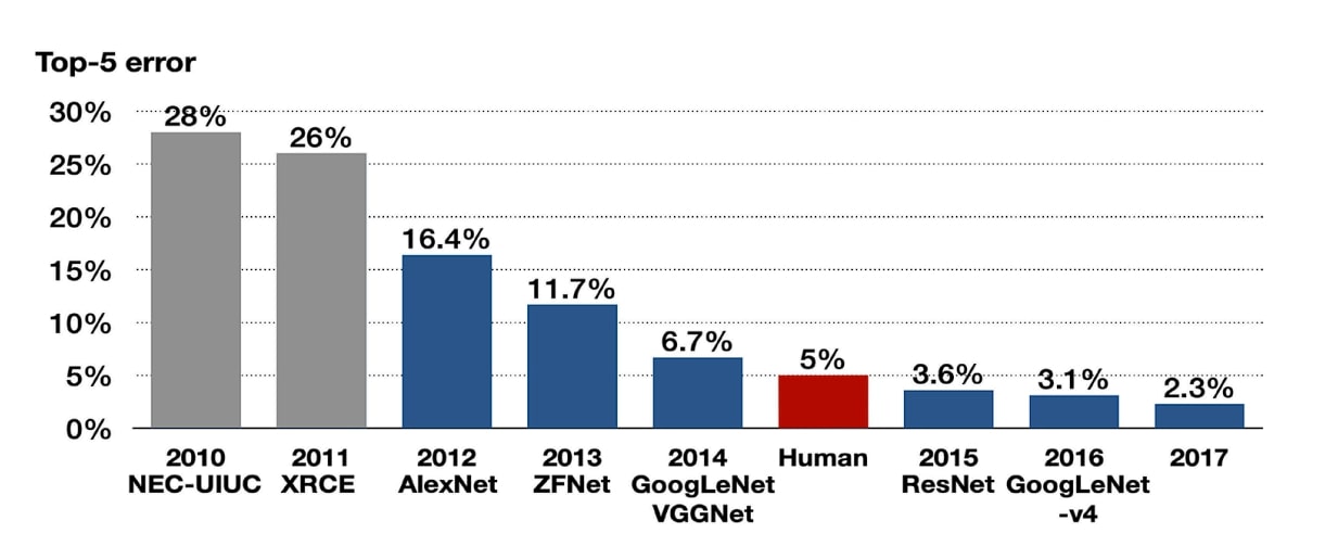
AlexNet proved that deep learning works at scale in 2012, sparking a race to improve CNN architectures. But simply adding more layers didn’t work. Networks deeper than 20 layers degraded during training, computational costs exploded, and memory constraints limited model size.
The innovations we’ll explore emerged as solutions to these challenges. Each architecture addressed specific problems while introducing ideas that influenced everything that followed. This is not a random collection of models, but a coherent story of progress through clever problem-solving.

Challenge 1: Going Deeper (VGG, 2014)
AlexNet demonstrated the power of depth with 8 layers. But could we go deeper? By 2014, researchers at Oxford’s Visual Geometry Group posed this question directly.
The Depth Hypothesis
The intuition was compelling. Deeper networks should learn more complex representations, with early layers detecting simple edges and colors, middle layers combining these into textures and parts, and deep layers recognizing complete objects and scenes. More layers mean more abstraction.
So why couldn’t we just keep stacking layers? Training deep networks in 2014 remained difficult. Gradients vanished, training took weeks, and most researchers stuck with networks under 20 layers.
VGG’s Answer: Stacked 3×3 Convolutions
VGGNet demonstrated that systematic depth works (Simonyan and Zisserman 2014). The key insight was using small 3×3 convolutions exclusively, stacked together to build deep networks.

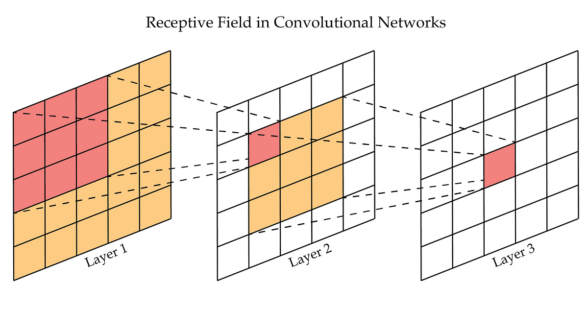
Why stack 3×3 filters instead of using larger filters? Consider the receptive field. Two 3×3 convolutions have the same receptive field as one 5×5 convolution (both see a 5×5 region of the input). But the stacked version has fewer parameters.
For a single 5×5 convolution:
\text{parameters} = 5 \times 5 = 25
For two stacked 3×3 convolutions:
\text{parameters} = 2 \times (3 \times 3) = 18
This yields a 28% parameter reduction while adding an extra ReLU nonlinearity between the layers, allowing the network to learn more complex functions.

The Architecture Pattern
VGG introduced a clean, systematic pattern that influenced all subsequent architectures.
After each pooling layer, double the channels:
\text{channels} = \{64 \to 128 \to 256 \to 512 \to 512\}
Spatial dimensions halve:
\text{spatial dimensions} = \{224 \to 112 \to 56 \to 28 \to 14 \to 7\}
This creates a pyramid structure where computational cost per layer stays roughly constant. As spatial dimensions decrease, increasing channel depth compensates by expanding representational capacity.
VGG16 (16 layers) and VGG19 (19 layers) achieved strong results on ImageNet. This validated that systematic depth improves accuracy. The architecture’s simplicity made it easy to understand and implement, contributing to its widespread adoption.
The Limitation
VGG16 contains approximately 140 million parameters, with the majority (102 million) concentrated in the first fully connected layer. This massive parameter count means training requires significant computational resources, inference is memory-intensive, and the model is prone to overfitting without strong regularization. The question became: can we achieve similar accuracy with fewer parameters?
Challenge 2: Computing Efficiently (Inception/GoogLeNet, 2014)
While VGG pushed depth systematically, researchers at Google asked a different question: how do we capture multi-scale features efficiently?
Multi-Scale Feature Extraction
Look at a photograph. Some objects are large and occupy significant image area, while others are small details. To recognize both, the network needs to examine features at multiple scales simultaneously. Traditional CNN layers use a single kernel size (like 3×3), but the optimal kernel size varies by context. Large kernels capture broad patterns while small kernels detect fine details. Inception’s answer: use multiple kernel sizes in parallel within the same layer (Szegedy et al. 2015).
The 1×1 Convolution Trick
Running multiple large convolutions in parallel is computationally expensive. Inception solves this through 1×1 convolutions for channel dimensionality reduction. At first, 1×1 convolutions seem strange. They don’t look at neighboring pixels, only at different channels at the same location, but this is precisely their power. They compress information across channels before applying larger, more expensive filters.
Consider a 3×3 convolution on a 256-channel feature map producing 256 output channels:
\text{parameters (without reduction)} = 3 \times 3 \times 256 \times 256 = 589{,}824
With a 1×1 convolution reducing to 64 channels first:
\text{parameters (with reduction)} = (1 \times 1 \times 256 \times 64) + (3 \times 3 \times 64 \times 256) = 163{,}840
This achieves a 72% parameter reduction while maintaining similar expressive power. The theoretical motivation behind 1×1 convolutions is elegant: Inception approximates sparse connectivity since not every pixel needs to connect to every pixel in the next layer. The 1×1 convolutions sparsify connections efficiently by operating primarily across channels rather than spatial dimensions.
The Inception Module
Each Inception module contains four parallel branches:
- 1×1 convolution: Captures point-wise patterns
- 1×1 → 3×3 convolution: Captures medium-scale patterns (with reduction)
- 1×1 → 5×5 convolution: Captures large-scale patterns (with reduction)
- 3×3 max pooling → 1×1 convolution: Preserves spatial structure differently
These branches process the same input simultaneously, and their outputs concatenate along the channel dimension to create a multi-scale representation. Mathematically, for input X:
Y_{\text{inception}} = \text{Concat}\big(Y_{1\times1}, \,Y_{3\times3}, \,Y_{5\times5}, \,Y_{\text{pool}}\big)
where each Y represents the output of its respective branch.
Global Average Pooling
VGG’s fully connected layers contain 102 million parameters. How do we eliminate this bottleneck? Inception uses global average pooling (Lin, Chen, and Yan 2013), taking the average value of each channel across all spatial positions instead of flattening feature maps and passing through dense layers. For a feature map with 1000 channels, this produces a 1000-dimensional vector directly, regardless of spatial size. This drastically reduces parameters (no heavy fully connected layers), creates translation invariance (averaging eliminates spatial dependence), and reduces overfitting risk.
Auxiliary Classifiers
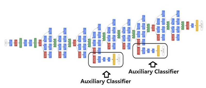
GoogLeNet introduced auxiliary classifiers at intermediate layers to combat vanishing gradients in deep networks. These classifiers attach to middle layers, computing losses that provide additional gradient signals during backpropagation. During training, the total loss combines the main classifier loss with auxiliary losses (typically weighted at 0.3), but at inference only the main classifier is used.

The Impact
GoogLeNet achieved accuracy comparable to VGG with 12× fewer parameters, demonstrating that architecture efficiency matters as much as depth. Later versions pushed these ideas further: Inception v2/v3 added batch normalization and factorized larger filters (5×5 became two 3×3 convolutions), Inception v4 integrated with residual connections, and Xception used depthwise separable convolutions. Batch Normalization, introduced around this time (Ioffe and Szegedy 2015), normalizes layer activations to zero mean and unit variance, stabilizing training and allowing higher learning rates. It became standard in nearly all subsequent architectures.
Challenge 3: Training Very Deep Networks (ResNet, 2015)
By 2015, researchers wanted networks with 50, 100, or even 150 layers. But a puzzling phenomenon blocked progress: networks deeper than about 20 layers exhibited degradation.
The Degradation Problem
Here’s what was strange: adding more layers to a working network increased training error (not test error, which would indicate overfitting, but training error itself). A deeper network could theoretically learn the identity function for extra layers, matching the shallower network’s performance, but in practice optimization failed. The deeper network couldn’t even learn to copy what the shallower network already achieved, revealing a fundamental optimization difficulty beyond vanishing gradients (which batch normalization addressed).
The Residual Learning Solution
Microsoft Research proposed an elegant solution: skip connections (He et al. 2015).
Instead of learning a direct mapping H(\mathbf{x}) from input \mathbf{x} to output, learn the residual F(\mathbf{x}) = H(\mathbf{x}) - \mathbf{x}. Then add the input back:
H(\mathbf{x}) = F(\mathbf{x}) + \mathbf{x}

Why does this help? If the optimal mapping is close to identity (the layer isn’t very useful), the network can easily learn F(\mathbf{x}) \approx 0 by pushing weights toward zero, while the skip connection ensures input information flows through unchanged. If a more complex transformation is needed, F(\mathbf{x}) can still learn it since the skip connection doesn’t constrain what the block can represent. It just makes optimization easier by providing a gradient highway during backpropagation.
Ensemble-Like Gradient Flow
Skip connections create multiple paths for gradients to flow backward. Some paths go through all convolutions. Others skip multiple blocks via cascaded skip connections. This ensemble of paths accelerates training and prevents vanishing gradients (Veit, Wilber, and Belongie 2016).

Bottleneck Blocks for Deeper Networks
ResNet-50, -101, and -152 use bottleneck blocks to maintain efficiency:
- 1×1 convolution: Reduces channel dimension (e.g., 256 → 64)
- 3×3 convolution: Operates on reduced dimension
- 1×1 convolution: Restores dimension (e.g., 64 → 256)

This shrinks the intermediate feature map, dramatically reducing computational cost while maintaining representational capacity through a design inspired by Inception’s bottleneck idea.
The Results
ResNet achieved:
- 152 layers trained successfully without degradation
- Top-5 error of 3.57% on ImageNet (better than human performance on the test set)
- Widespread adoption across computer vision tasks
The impact extended beyond CNNs. Skip connections appeared in:
- U-Net for medical image segmentation
- DenseNet which connects every layer to every other layer
- Transformers for natural language processing
- Nearly all modern deep architectures
ResNet showed that with the right architecture, depth isn’t a limitation. It’s a resource.
ResNeXt: Width Through Cardinality
ResNeXt (Xie et al. 2017) extended ResNet by increasing network width through grouped convolutions rather than just adding depth or channels. The idea is to split the bottleneck convolution path into multiple parallel groups (typically 32), each processing independently, then aggregate their outputs through concatenation or addition.

This “cardinality” dimension provides another axis for scaling networks. ResNeXt achieves better accuracy than ResNet at similar computational cost by increasing cardinality instead of just going deeper.
Challenge 4: Global Context (Vision Transformer, 2020)
CNNs build global understanding slowly through stacked local operations, with early layers seeing only small patches (3×3 or 5×5 regions) and deeper layers expanding the receptive field. Even in deep networks, truly global connections require many layers. What if we could capture global relationships immediately?
The Self-Attention Mechanism
Vision Transformers (ViT) replace convolution with self-attention, which computes relationships between all positions simultaneously. For each patch of the image, it determines which other patches are relevant, regardless of distance, providing immediate global context.
How does the mechanism work? Given input features X, compute three matrices through learned linear projections:
Q = XW_Q, \quad K = XW_K, \quad V = XW_V
where Q (queries), K (keys), and V (values) represent different views of the input.
Attention scores measure similarity between queries and keys:
\text{Attention}(Q, K, V) = \text{softmax}\left(\frac{QK^T}{\sqrt{d_k}}\right)V
This computes a weighted average of values, where weights depend on query-key similarity. Intuitively, each position “asks” (via its query) what information to gather from all other positions (via their keys), then aggregates their values accordingly.
Patches as Tokens
ViT treats images like text: divide the image into fixed-size patches (typically 16×16), flatten each patch into a vector, and treat these vectors as “tokens” (analogous to words in NLP). Add positional encodings to preserve spatial information (since self-attention is permutation-invariant) and pass through a standard Transformer encoder with multiple self-attention layers. A special CLS token prepended to the sequence gathers global information, and after all Transformer layers, the CLS token’s representation feeds into the classification head, mirroring how BERT processes text.
Trade-offs: Data and Compute
Vision Transformers achieve state-of-the-art accuracy on large datasets like ImageNet-21k (14 million images), but they have important trade-offs. They provide a global receptive field from the first layer, better scaling properties with dataset size, and a unified architecture for vision and language. However, they require more training data than CNNs due to less inductive bias, impose higher computational cost since self-attention is O(n^2) in sequence length, and prove less effective on small datasets without strong augmentation.
When should you use ViT versus CNNs? Use ViT when you have large datasets (millions of images), substantial computational resources, and tasks benefiting from global context like scene understanding or fine-grained classification. Use CNNs when you have limited data (thousands of images), constrained compute (edge devices, mobile), or tasks benefiting from spatial locality (object detection, segmentation).
Hybrid Approaches
Recent research combines CNN and Transformer strengths. The field continues evolving, blending ideas from both paradigms.
The Narrative of Progress
The thread connecting these innovations is clear. In 2012, AlexNet showed depth works but only to 8 layers. By 2014, VGG stacked small convolutions to go deeper (16-19 layers), while Inception used multi-scale features and 1×1 convolutions for efficiency. In 2015, ResNet’s skip connections enabled training very deep networks (152 layers). ResNeXt in 2017 increased width through cardinality, not just depth. Finally, Vision Transformers in 2020 replaced convolution with self-attention for global context.
Each innovation addressed limitations of its predecessors while preserving their insights. Modern architectures mix and match these ideas: residual connections for depth, multi-scale features for efficiency, attention for global context.
Choosing the Right Architecture
For your next computer vision project, which architecture should you choose? ResNet-50 is the default choice, offering an excellent accuracy-computational cost trade-off with widely available pre-trained weights that work well across diverse tasks. EfficientNet matters when deployment efficiency is critical, carefully balancing depth, width, and resolution for optimal accuracy per parameter, while MobileNet and EfficientNet-Lite serve mobile and edge devices by sacrificing some accuracy for fast inference and small model size. Vision Transformer (ViT) excels when you have large datasets (millions of images) and substantial compute, delivering state-of-the-art accuracy on challenging benchmarks, while Swin Transformer provides Transformer benefits with more reasonable compute requirements, proving especially good for dense prediction tasks. Start with ResNet-50 for strong performance across almost all applications, then optimize later if specific constraints (speed, memory, accuracy) demand it.
Summary
We traced CNN evolution through successive innovations solving specific challenges. VGG demonstrated that depth matters through stacked 3×3 convolutions, while Inception showed how to capture multi-scale features efficiently using 1×1 convolutions and parallel branches. ResNet enabled training very deep networks (152 layers) through skip connections that ease optimization and improve gradient flow. Vision Transformers replaced convolution with self-attention, trading inductive bias for global context at the cost of requiring more data and compute.
Each architecture built on its predecessors’ insights. Modern networks combine ideas from all of them: residual connections for depth, multi-scale features for efficiency, attention for global understanding. Architecture design is problem-solving. Understanding why these innovations emerged helps you make informed choices for your own applications.