Spatial Graph Networks
This module explores spatial approaches to graph convolution.
You’ll learn:
- How ChebNet bridges spectral and spatial domains using Chebyshev polynomials.
- How GCN achieves radical simplification through first-order approximation and renormalization.
- How GraphSAGE enables inductive learning through sampling and aggregation.
- How GAT learns to weight neighbors using attention mechanisms.
- How GIN achieves maximum discriminative power by preserving multiset information.
- Practical trade-offs between these architectures for different graph learning tasks.
From Spectral to Spatial
Let’s talk about why we need spatial methods. The spectral perspective offers mathematical elegance but faces practical challenges. Computing eigendecomposition scales poorly to large graphs. Spectral filters lack spatial locality, allowing distant nodes to directly influence each other.
What’s the alternative? Spatial methods take a different approach. Instead of transforming to frequency domains, they define convolution directly as aggregating features from local neighborhoods.
Think of it as message passing. Each node collects information from its neighbors, combines it, and produces an updated representation. This shift brings immediate benefits.
Spatial methods scale linearly with the number of edges. They preserve locality by design. They generalize naturally to unseen nodes. But we must carefully design how nodes aggregate neighbor information.
ChebNet: The Bridge
How do we bridge spectral and spatial perspectives? ChebNet (Defferrard, Bresson, and Vandergheynst 2016) achieves this using Chebyshev polynomials. The key insight is that we can approximate spectral filters without computing full eigendecompositions.
Let’s recall the learnable spectral filter:
{\bf L}_{\text{learn}} = \sum_{k=1}^K \theta_k {\bf u}_k {\bf u}_k^\top
ChebNet approximates this using Chebyshev polynomials of the scaled Laplacian \tilde{{\bf L}} = \frac{2}{\lambda_{\text{max}}}{\bf L} - {\bf I}:
{\bf L}_{\text{learn}} \approx \sum_{k=0}^{K-1} \theta_k T_k(\tilde{{\bf L}})
where T_k are Chebyshev polynomials defined recursively:
\begin{aligned} T_0(\tilde{{\bf L}}) &= {\bf I} \\ T_1(\tilde{{\bf L}}) &= \tilde{{\bf L}} \\ T_k(\tilde{{\bf L}}) &= 2\tilde{{\bf L}} T_{k-1}(\tilde{{\bf L}}) - T_{k-2}(\tilde{{\bf L}}) \end{aligned}
The convolution becomes:
{\bf x}^{(\ell+1)} = h\left( \sum_{k=0}^{K-1} \theta_k T_k(\tilde{{\bf L}}){\bf x}^{(\ell)}\right)
Why does this help? The crucial property is that multiplying by \tilde{{\bf L}} is a local operation. Computing T_k(\tilde{{\bf L}}){\bf x} only involves nodes within k hops of each neighborhood.
This achieves spatial locality without explicit eigendecomposition. ChebNet typically uses small K (e.g., K=3), limiting receptive fields to nearby neighbors. Deeper networks expand receptive fields by stacking layers.
GCN: Radical Simplification
Can we simplify further? While ChebNet offers principled spectral approximation, Kipf and Welling (2017) proposed an even simpler variant that became one of the most widely used graph neural networks.
First-Order Approximation
What’s the key departure? Using only the first-order Chebyshev approximation. Setting K=1 and making additional simplifications yields:
g_{\theta} * x \approx \theta({\bf I}_N + {\bf D}^{-\frac{1}{2}}{\bf A}{\bf D}^{-\frac{1}{2}})x
where {\bf D} is the degree matrix and {\bf A} is the adjacency matrix. This leaves a single learnable parameter \theta instead of K parameters. Notice the dramatic reduction in complexity.
Renormalization Trick
How do we stabilize training in deep networks? GCN adds self-loops to the graph:
\tilde{{\bf A}} = {\bf A} + {\bf I}_N, \quad \tilde{{\bf D}}_{ii} = \sum_j \tilde{{\bf A}}_{ij}
This ensures each node includes its own features when aggregating from neighbors, preventing information loss and mitigating gradient vanishing.
Layer-Wise Propagation
The final GCN layer becomes remarkably simple:
{\bf X}^{(\ell+1)} = \sigma(\tilde{{\bf D}}^{-\frac{1}{2}}\tilde{{\bf A}}\tilde{{\bf D}}^{-\frac{1}{2}}{\bf X}^{(\ell)}{\bf W}^{(\ell)})
where {\bf X}^{(\ell)} \in \mathbb{R}^{N \times f_{\text{in}}} are node features at layer \ell, {\bf W}^{(\ell)} \in \mathbb{R}^{f_{\text{in}} \times f_{\text{out}}} is a learnable weight matrix, and \sigma is a nonlinear activation. Look at how simple this formula is compared to spectral methods.
Despite its simplicity, GCN achieves strong performance on many tasks. The symmetric normalization \tilde{{\bf D}}^{-\frac{1}{2}}\tilde{{\bf A}}\tilde{{\bf D}}^{-\frac{1}{2}} ensures numerical stability by normalizing message magnitudes.
Implement a simple GCN model for node classification. Coding Exercise
GraphSAGE: Sample and Aggregate
What about scalability? GCN processes entire graphs at once, limiting its applicability to large graphs. GraphSAGE (Hamilton, Ying, and Leskovec 2017) introduced an inductive framework that generates embeddings by sampling and aggregating features from neighborhoods.
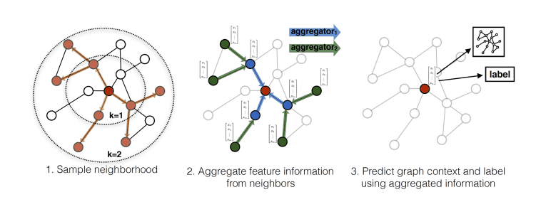
Neighborhood Sampling
Instead of using all neighbors, GraphSAGE samples a fixed-size set. This controls memory complexity and enables handling dynamic graphs where new nodes arrive continuously.
Consider a growing citation network. Traditional GCNs require recomputing filters for the entire graph with each new paper. GraphSAGE generates embeddings for new nodes by sampling their neighbors, without retraining. This is what we mean by inductive learning.
Aggregation Functions
How does GraphSAGE combine information? It distinguishes self-information from neighborhood information. First, aggregate neighbor features:
{\bf h}_{\mathcal{N}(v)} = \text{AGGREGATE}(\{{\bf h}_u, \forall u \in \mathcal{N}(v)\})
Common aggregators include mean, max-pooling, and LSTM. The mean aggregator computes \text{mean}(\{{\bf h}_u, \forall u \in \mathcal{N}(v)\}). Max-pooling uses \max(\{\sigma({\bf W}_{\text{pool}}{\bf h}_u + {\bf b}), \forall u \in \mathcal{N}(v)\}). LSTM applies to randomly permuted neighbors.
Then concatenate self and neighborhood information:
{\bf z}_v = \text{CONCAT}({\bf h}_v, {\bf h}_{\mathcal{N}(v)})
Normalize and apply the learned transformation:
{\bf h}_v^{(\ell+1)} = \sigma({\bf W}^{(\ell)} \frac{{\bf z}_v}{\|{\bf z}_v\|_2})
This explicit separation allows the model to learn how much to trust self versus neighbors.
GAT: Learning Attention
Here’s a crucial question. Should all neighbors contribute equally? Graph Attention Networks (velickovic2018graph?) let the model learn which neighbors matter most.
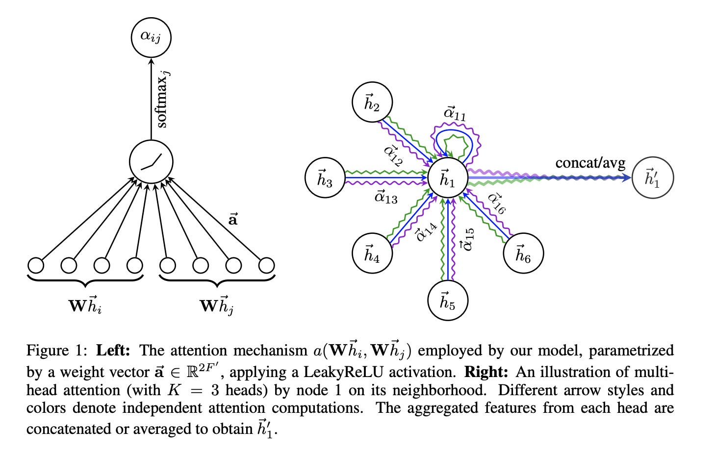
Attention Mechanism
How does attention work? GAT computes attention weights \alpha_{ij} indicating how much node i should attend to node j:
\alpha_{ij} = \frac{\exp(e_{ij})}{\sum_{k \in \mathcal{N}(i)} \exp(e_{ik})}
where e_{ij} measures edge importance. How do we compute edge importance? One approach uses a neural network with shared parameters. First, transform node features: \tilde{{\bf h}}_i = {\bf W}{\bf h}_i. Then compute attention logits: e_{ij} = \text{LeakyReLU}({\bf a}^T[\tilde{{\bf h}}_i \| \tilde{{\bf h}}_j]).
Here {\bf a} is a learnable attention vector and \| denotes concatenation.
Node Update
With attention weights, the update becomes a weighted sum:
{\bf h}_i^{(\ell+1)} = \sigma\left(\sum_{j \in \mathcal{N}(i) \cup \{i\}} \alpha_{ij}{\bf W}_{\text{feature}}{\bf h}_j^{(\ell)}\right)
Multi-Head Attention
How do we stabilize training? GAT uses multiple attention heads and concatenates outputs:
{\bf h}_i^{(\ell+1)} = \|_{k=1}^K \sigma\left(\sum_{j \in \mathcal{N}(i) \cup \{i\}} \alpha_{ij}^k{\bf W}^k{\bf h}_j^{(\ell)}\right)
Different heads can focus on different aspects of neighborhood structure. This is similar to multi-head attention in Transformers.
GIN: The Power of Aggregation
Let’s ask a fundamental question. What is the maximum discriminative power of graph neural networks? Graph Isomorphism Networks (Xu et al. 2019) provide an answer.
The Weisfeiler-Lehman Test
The Weisfeiler-Lehman (WL) test determines if two graphs are structurally identical. It iteratively refines node labels by hashing neighbor labels.
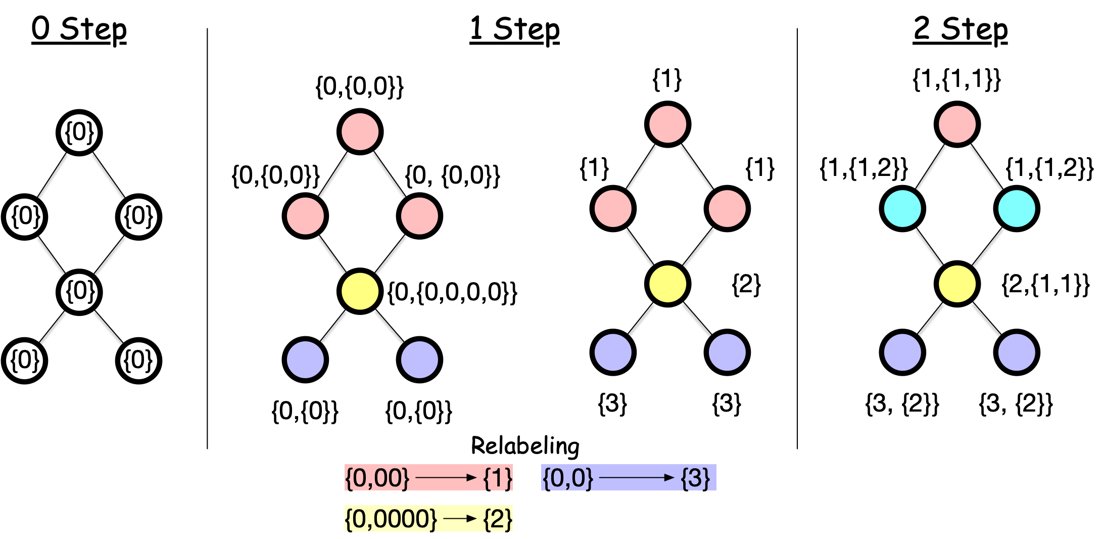
How does the process work? First, assign all nodes the same initial label. For each node, collect neighbor labels and create a multiset. Hash the multiset with the node’s own label to produce a new label. Repeat until convergence.
Two graphs are isomorphic if they have identical label distributions after convergence. The WL test fails on some graphs (like regular graphs) but works well in practice. The standard WL test is called 1-WL, while higher-order variants exist that can distinguish more graphs, leading to more powerful GNNs.
GIN’s Key Insight
What’s the connection between WL and GNNs? The parallel is striking. WL iteratively aggregates neighbor labels via hash function. GNNs iteratively aggregate neighbor features via learned function.
What’s the crucial difference? Discriminative power. WL’s hash function always distinguishes different neighbor multisets by counting occurrences. Common GNN aggregators like mean or max can fail. If all neighbors have identical features, these aggregators produce the same output regardless of neighborhood size.
How does GIN solve this? By designing an aggregation that preserves multiset information:
{\bf h}_v^{(k+1)} = \text{MLP}^{(k)}\left((1 + \epsilon^{(k)}) \cdot {\bf h}_v^{(k)} + \sum_{u \in \mathcal{N}(v)} {\bf h}_u^{(k)}\right)
where \text{MLP}^{(k)} is a multi-layer perceptron and \epsilon^{(k)} is a learnable or fixed scalar. Why does this work?
The sum aggregation preserves multiset information. The self-loop with weight (1 + \epsilon) distinguishes nodes from their neighborhoods. The MLP provides sufficient capacity to approximate injective functions, matching WL’s discriminative power.
Xu et al. (2019) prove that GIN can distinguish any graphs that WL can distinguish. This makes it maximally powerful within the class of message-passing neural networks.
Comparing Approaches
Let’s compare what we’ve learned. We have seen five spatial architectures, each with distinct design choices.
| Method | Key Innovation | Trade-off |
|---|---|---|
| ChebNet | Chebyshev approximation | Bridges spectral/spatial, moderate complexity |
| GCN | Radical simplification | Simple, efficient, strong baseline |
| GraphSAGE | Sampling + separation | Scalable, inductive, flexible |
| GAT | Learned attention | Interpretable, handles heterophily |
| GIN | Injective aggregation | Maximum discriminative power |
Which one should you use? The best choice depends on your task. GCN provides a strong baseline. GraphSAGE handles large, dynamic graphs. GAT works when neighbor importance varies. GIN excels at graph-level tasks requiring fine-grained discrimination.
All these methods share a common theme. They define convolution as neighborhood aggregation, preserving spatial locality while learning which patterns matter for downstream tasks. This is the essence of spatial graph neural networks.
What comes next? In Part 4, we shift from node classification to representation learning. We explore graph embeddings that map nodes to continuous vector spaces, enabling clustering, visualization, and transfer learning across tasks.