import numpy as np
import matplotlib.pyplot as plt
import gensim.downloader as api

# Download and load pre-trained GloVe embeddings
model = api.load("glove-wiki-gigaword-100")SemAxis: Meaning as Direction
What you’ll learn in this module
This module introduces SemAxis, a framework for measuring semantic meaning through contrast.
You’ll learn:
- How meaning emerges from contrast rather than inherent properties.
- How to construct semantic axes by subtracting antonym vectors.
- How to project words onto axes to measure alignment with concepts like sentiment or intensity.
- How to build robust axes using centroids of synonym clusters.
- How to visualize semantic relationships in 2D space by crossing two axes.
Embedding Space as Contrast
Have you ever wondered how to extract specific meanings from word embeddings? We intuitively treat word embeddings as static maps where “king” is simply near “queen”, assuming the meaning is inherent to the coordinate itself, much like a city has a fixed latitude and longitude. This is a convenient fiction. In embedding space, meaning emerges entirely from contrast.
SemAxis defines a semantic axis by subtracting one vector from its opposite (e.g., v_{good} - v_{bad}), isolating a single semantic dimension that ignores all other information.
Given two pole words w_+ and w_-, the axis is defined as:
v_{\text{axis}} = \frac{v_{w_+} - v_{w_-}}{||v_{w_+} - v_{w_-}\||_2}
The denominator is the L_2 norm of the difference vector, ensuring v_{\text{axis}} is a unit vector. Using this “ruler”, we project words onto the axis with cosine similarity between v_{w} and v_{\text{axis}}:
\text{Position of w on axis } v_{\text{axis}} = \cos(v_{\text{axis}},v_{w})
Let’s build a “Sentiment Compass” to measure the emotional charge of words that aren’t explicitly emotional. First, we load the standard GloVe embeddings.
Defining the Axis
We define the axis not as a point, but as the difference vector between two poles. This vector points from “bad” to “good”.
def create_axis(pos_word, neg_word, model):
    return model[pos_word] - model[neg_word]


# The "Sentiment" Axis
sentiment_axis = create_axis("good", "bad", model)
Measuring Alignment
How do we see where a word falls on this axis? We project it using the normalized dot product. If the vector points in the same direction, the score is positive; if it points away, it is negative.
def get_score(word, axis, model):
    v_word = model[word]
    # Cosine similarity is just a normalized dot product
    return np.dot(v_word, axis) / (np.linalg.norm(v_word) * np.linalg.norm(axis))


words = ["excellent", "terrible", "mediocre", "stone", "flower"]
for w in words:
    print(f"{w}: {get_score(w, sentiment_axis, model):.3f}")
excellent: 0.523
terrible: -0.208
mediocre: -0.001
stone: 0.181
flower: 0.204Robustness via Centroids
Single words are noisy since “bad” might carry connotations of “naughty” or “poor quality”. The solution is to use the centroid of a cluster of synonyms, averaging out the noise to leave only the pure semantic signal.
def create_robust_axis(pos_word, neg_word, model, k=5):
    # Get k nearest neighbors for both poles
    pos_group = [pos_word]
    pos_words = model.most_similar(pos_word, topn=k)
    for word, _ in pos_words:
        pos_group.append(word)

    neg_group = [neg_word]
    neg_words = model.most_similar(neg_word, topn=k)
    for word, _ in neg_words:
        neg_group.append(word)

    # Average them to find the centroid
    pos_vec = np.mean([model[w] for w in pos_group], axis=0)
    neg_vec = np.mean([model[w] for w in neg_group], axis=0)

    return pos_vec - neg_vec


robust_axis = create_robust_axis("good", "bad", model)
The 2D Semantic Space
When does the real power emerge? When we cross two axes, plotting words against “Sentiment” and “Intensity” (Strong vs. Weak) to reveal relationships that a single list hides.
Code
def plot_2d(words, axis_x, axis_y, model):
    x_scores = [get_score(w, axis_x, model) for w in words]
    y_scores = [get_score(w, axis_y, model) for w in words]

    plt.figure(figsize=(5, 5))
    plt.scatter(x_scores, y_scores)

    for i, w in enumerate(words):
        plt.annotate(
            w,
            (x_scores[i], y_scores[i]),
            xytext=(5, 5),
            textcoords="offset points",
            fontsize=16,
        )

    plt.axhline(0, color="k", alpha=0.3)
    plt.axvline(0, color="k", alpha=0.3)
    plt.xlabel("Sentiment (Bad -> Good)")
    plt.ylabel("Intensity (Weak -> Strong)")
    plt.show()


intensity_axis = create_axis("strong", "weak", model)
test_words = [
    "excellent",
    "terrible",
    "mediocre",
    "mild",
    "extreme",
    "murder",
    "charity",
]

plot_2d(test_words, sentiment_axis, intensity_axis, model)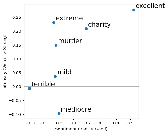
The Key Insight
To define a concept, you must first define its opposite. Meaning isn’t stored in the word itself but lives in the contrast space, where the relationship between poles defines an axis. SemAxis operationalizes this principle, isolating the dimension that matters by defining opposition.