The Spectral Perspective

What you’ll learn in this module

This module introduces the spectral approach to graph convolution.

You’ll learn:

• How to define frequency for graph signals using the Laplacian matrix.
• Why eigenvectors act as basis functions and eigenvalues measure roughness.
• How to design spectral filters that control which frequencies pass through.
• How to build learnable spectral graph convolutional networks.
• The computational limitations that motivate spatial methods.

Finding Frequency in Graphs

Images live in a spatial domain, but the Fourier transform reveals their frequency content. Low frequencies capture smooth gradients and overall structure. High frequencies capture sharp edges and fine details.

Graphs need their own notion of frequency. Consider a network of nodes where each node has a feature value. What makes a signal “smooth” on a graph?

Intuitively, smoothness means connected nodes have similar values. Roughness means neighbors differ significantly. Let’s formalize this intuition.

Total Variation: Measuring Roughness

Consider a network of N nodes where each node i has a scalar feature x_i \in \mathbb{R}. Define the total variation as:

J = \frac{1}{2}\sum_{i=1}^N\sum_{j=1}^N A_{ij}(x_i - x_j)^2

where A_{ij} is the adjacency matrix. This quantity sums the squared differences between connected nodes.

Small J means smooth variation (low frequency). Large J means rough variation (high frequency).

We can rewrite J in matrix form. Through algebraic manipulation, we obtain:

J = {\bf x}^\top {\bf L} {\bf x}

where {\bf x} = [x_1, x_2, \ldots, x_N]^\top and {\bf L} is the graph Laplacian:

L_{ij} = \begin{cases} k_i & \text{if } i = j \\ -1 & \text{if } i \text{ and } j \text{ are connected} \\ 0 & \text{otherwise} \end{cases}

with k_i being the degree of node i.

Detailed derivation

Starting from the definition of total variation:

\begin{aligned} J &= \frac{1}{2}\sum_{i=1}^N\sum_{j=1}^N A_{ij}(x_i - x_j)^2 \\ &= \frac{1}{2}\sum_{i=1}^N\sum_{j=1}^N A_{ij}(x_i^2 + x_j^2 - 2x_ix_j) \\ &= \sum_{i=1}^N x_i^2 \sum_{j=1}^N A_{ij} - \sum_{i=1}^N\sum_{j=1}^N A_{ij}x_ix_j \\ &= \sum_{i=1}^N x_i^2 k_i - \sum_{i=1}^N\sum_{j=1}^N A_{ij}x_ix_j \\ &= {\bf x}^\top {\bf D} {\bf x} - {\bf x}^\top {\bf A} {\bf x} \\ &= {\bf x}^\top ({\bf D} - {\bf A}) {\bf x} \\ &= {\bf x}^\top {\bf L} {\bf x} \end{aligned}

where {\bf D} is the diagonal degree matrix with D_{ii} = k_i.

The Laplacian {\bf L} plays the same role for graphs that the derivative operator plays for continuous signals. It measures how much a signal varies across edges.

Eigenvectors as Basis Functions

In Fourier analysis, we decompose signals into sinusoidal basis functions. For graphs, eigenvectors of the Laplacian serve as basis functions. How does this work?

Consider the eigendecomposition of {\bf L}:

{\bf L} = \sum_{i=1}^N \lambda_i {\bf u}_i {\bf u}_i^\top

where \lambda_i are eigenvalues and {\bf u}_i are eigenvectors. We can decompose the total variation J as:

J = {\bf x}^\top {\bf L} {\bf x} = \sum_{i=1}^N \lambda_i ({\bf x}^\top {\bf u}_i)^2

Each term ({\bf x}^\top {\bf u}_i)^2 measures how much signal {\bf x} aligns with eigenvector {\bf u}_i. The eigenvalue \lambda_i weights this contribution.

What do eigenvalues tell us? Compute the total variation of eigenvector {\bf u}_i itself:

J_i = {\bf u}_i^\top {\bf L} {\bf u}_i = \lambda_i

This reveals the key insight. Eigenvalues measure the total variation of their corresponding eigenvectors. Small eigenvalues correspond to smooth eigenvectors (low frequency). Large eigenvalues correspond to rough eigenvectors (high frequency).

Now consider any signal {\bf x}. If {\bf x} aligns strongly with a low-eigenvalue eigenvector, {\bf x} is smooth. If {\bf x} aligns with a high-eigenvalue eigenvector, {\bf x} is rough.

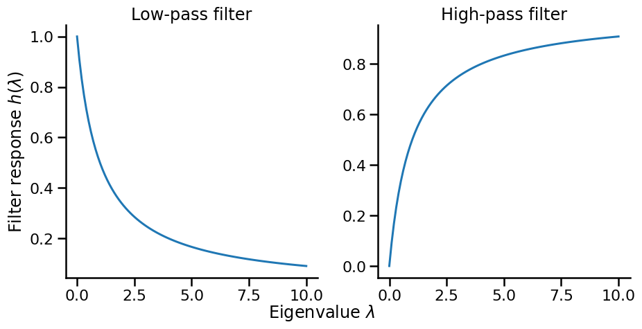
Spectral Filtering

Eigenvalues act as natural filters. We can design custom filters h(\lambda_i) to control which frequencies pass through. Let’s look at two fundamental filters.

Low-pass Filter (smoothing): h_{\text{low}}(\lambda) = \frac{1}{1 + \alpha\lambda}

This suppresses high frequencies (large \lambda) and preserves low frequencies (small \lambda), resulting in smoother signals.

High-pass Filter (edge detection): h_{\text{high}}(\lambda) = \frac{\alpha\lambda}{1 + \alpha\lambda}

This suppresses low frequencies and emphasizes high frequencies. The result highlights rapid variations like boundaries between communities.

The parameter \alpha controls the filter’s strength. Larger \alpha makes the transition between frequencies sharper.

Learnable Spectral Filters

Hand-designed filters work for specific tasks, but what if we want to learn filters from data? This question leads to spectral graph convolutional networks.

The simplest learnable filter uses a linear combination of eigenvectors:

{\bf L}_{\text{learn}} = \sum_{k=1}^K \theta_k {\bf u}_k {\bf u}_k^\top

where \theta_k are learnable parameters and K is the filter rank. Instead of fixed weights \lambda_k, we learn weights \theta_k that maximize performance on downstream tasks. This shifts from hand-designed to data-driven filters.

Building on this idea, Bruna et al. (2014) proposed spectral convolutional neural networks by adding nonlinearity:

{\bf x}^{(\ell+1)} = h\left( {\bf L}_{\text{learn}} {\bf x}^{(\ell)}\right)

where h is an activation function (e.g., ReLU) and {\bf x}^{(\ell)} is the feature vector at layer \ell.

For multidimensional features {\bf X} \in \mathbb{R}^{N \times f_{\text{in}}}, we extend this to produce outputs {\bf X}' \in \mathbb{R}^{N \times f_{\text{out}}}:

{\bf X}^{(\ell+1)}_j = h\left( \sum_{i=1}^{f_{\text{in}}} {\bf L}_{\text{learn}}^{(i,j)} {\bf X}^{(\ell)}_i\right)

where {\bf L}_{\text{learn}}^{(i,j)} = \sum_{k=1}^K \theta_{k, (i,j)} {\bf u}_k {\bf u}_k^\top is a separate learnable filter for each input-output dimension pair.

This architecture stacks multiple layers, each learning which spectral components matter for the task. Deeper layers capture increasingly complex patterns.

The Computational Challenge

Spectral methods face two critical limitations. What are they?

Computational cost: Computing eigendecomposition requires \mathcal{O}(N^3) operations, prohibitive for large graphs with millions of nodes.

Lack of spatial locality: Learned filters operate on all eigenvectors, meaning every node can influence every other node. This loses the inductive bias of locality that makes CNNs powerful.

These limitations motivated the development of spatial methods. Spatial approaches define convolution directly in the graph domain without requiring eigendecomposition. We explore this alternative in the next part.

Key Takeaways

The spectral perspective reveals that graphs have frequency domains. The Laplacian’s eigenvectors serve as basis functions, and eigenvalues indicate how rapidly signals vary.

Spectral filters control which frequencies pass through. We can learn these filters for specific tasks. This mathematical elegance comes at a cost.

Eigendecomposition is expensive, and spectral filters lack spatial locality. But the insights gained inform spatial methods. In Part 3, we see how spatial methods address these limitations while preserving the power of learned graph convolution.

References

Bruna, Joan, Wojciech Zaremba, Arthur Szlam, and Yann LeCun. 2014. “Spectral Networks and Locally Connected Networks on Graphs.” In 2nd International Conference on Learning Representations, ICLR 2014, Banff, AB, Canada, April 14-16, 2014, Conference Track Proceedings, edited by Yoshua Bengio and Yann LeCun. http://arxiv.org/abs/1312.6203.