Show image display code
# Display the image
plt.figure(figsize=(8, 6))
plt.imshow(img_array)
plt.title("Original Image")
plt.axis("off")
plt.show()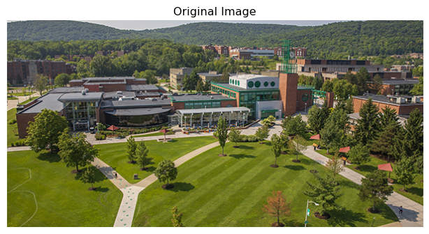
This section introduces images as structured data.
You’ll learn:
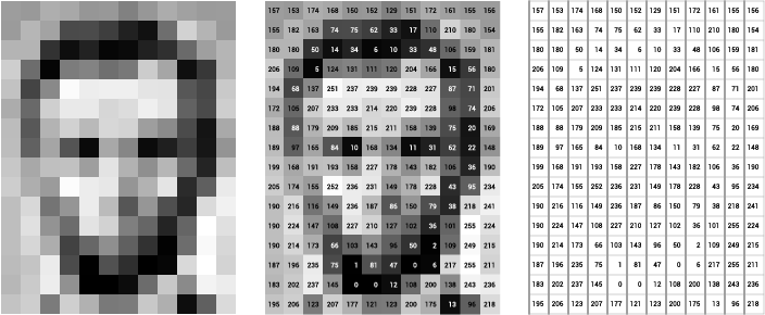
Let’s talk about what an image really is from a computer’s perspective. When you look at a photograph, you see faces, objects, and scenes, but to a machine, that same photograph is simply a grid of numbers where each value represents the brightness or color at a specific location. How can numbers capture the richness of visual information? The answer lies in spatial structure. Unlike a spreadsheet where row order doesn’t matter, the arrangement of numbers in an image is everything, with neighboring pixels relating to each other to form edges, textures, and patterns.
The very first step in understanding images is to examine the grayscale case, where an image contains only brightness information with no color. We can think of it as a 2D matrix where each entry is a pixel intensity value. Consider a tiny 6×6 grayscale image:
X = \begin{bmatrix} 10 & 10 & 80 & 10 & 10 & 10 \\ 10 & 10 & 80 & 10 & 10 & 10 \\ 10 & 10 & 80 & 10 & 10 & 10 \\ 10 & 10 & 80 & 10 & 10 & 10 \\ 10 & 10 & 80 & 10 & 10 & 10 \\ 10 & 10 & 80 & 10 & 10 & 10 \end{bmatrix}
Here, the value 10 represents dark pixels, while 80 represents bright pixels. The third column forms a bright vertical line. This simple example shows how spatial patterns emerge from the arrangement of numbers.
Let’s make this concrete by loading an actual image and examining its structure. We’ll use Python with standard libraries to see what an image really looks like under the hood.
# Display the image
plt.figure(figsize=(8, 6))
plt.imshow(img_array)
plt.title("Original Image")
plt.axis("off")
plt.show()
# Examine the image properties
print(f"Image shape: {img_array.shape}")
print(f"Data type: {img_array.dtype}")
print(f"Value range: [{img_array.min()}, {img_array.max()}]")
Image shape: (300, 600, 3)
Data type: uint8
Value range: [0, 255]What does the shape tell us? The output (height, width, 3) reveals three dimensions: the first two specify spatial location, while the third holds three color channels. Let’s zoom into a small patch to see the actual numbers:
# Extract a tiny 5x5 patch from the center
center_y, center_x = img_array.shape[0] // 2, img_array.shape[1] // 2
patch = img_array[center_y:center_y+5, center_x:center_x+5, 0]  # Red channel only

print("A 5x5 patch of pixel values (Red channel):")
print(patch)
A 5x5 patch of pixel values (Red channel):
[[ 45 49 40 93 141]
[ 55 52 55 113 102]
[ 35 46 63 121 104]
[136 52 48 84 124]
[225 90 41 73 136]]These are the actual numbers the computer sees. Each value between 0 and 255 represents brightness in the red channel for that pixel location.
Color images extend the grayscale concept by using three separate matrices, one for each color channel: Red, Green, and Blue (RGB). Think of these as three grayscale images stacked on top of each other. When you combine the values from all three channels at a given location, you get the color for that pixel: [255, 0, 0] is pure red, [0, 255, 0] is pure green, and [255, 255, 255] is white. How do the channels look separately? Let’s visualize them:
fig, axes = plt.subplots(1, 4, figsize=(16, 4))

# Original image
axes[0].imshow(img_array)
axes[0].set_title("Original Image")
axes[0].axis("off")

# Individual channels
channel_names = ['Red', 'Green', 'Blue']
colors = ['Reds', 'Greens', 'Blues']

for i, (name, cmap) in enumerate(zip(channel_names, colors)):
    axes[i+1].imshow(img_array[:, :, i], cmap=cmap)
    axes[i+1].set_title(f"{name} Channel")
    axes[i+1].axis("off")

plt.tight_layout()
plt.show()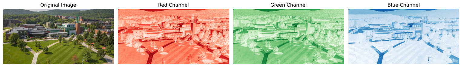
Notice how each channel emphasizes different aspects of the scene. The red channel might be bright where red objects appear, while the blue channel highlights sky and water.
Shift your attention from individual pixel values to relationships between pixels. This is what makes images fundamentally different from tabular data: in a spreadsheet, you can shuffle the rows without losing information, but in an image, shuffling pixels destroys everything because the spatial arrangement is the information itself. An edge appears when neighboring pixels have very different values, a texture emerges from repeating patterns across nearby locations, and an object is a coherent region of similar pixels. Why does this matter for machine learning? Fully connected networks treat every input independently, ignoring spatial relationships, while convolutional networks (which we’ll explore soon) are designed specifically to exploit this structure.
Let’s practice manipulating image representations to build intuition:
# Convert to grayscale by averaging channels
grayscale = np.mean(img_array, axis=2).astype(np.uint8)

print(f"RGB shape: {img_array.shape}")
print(f"Grayscale shape: {grayscale.shape}")
RGB shape: (300, 600, 3)
Grayscale shape: (300, 600)# Create a side-by-side comparison
fig, axes = plt.subplots(1, 2, figsize=(12, 5))
axes[0].imshow(img_array)
axes[0].set_title("RGB Image (3 channels)")
axes[0].axis("off")
axes[1].imshow(grayscale, cmap='gray')
axes[1].set_title("Grayscale Image (1 channel)")
axes[1].axis("off")
plt.tight_layout()
plt.show()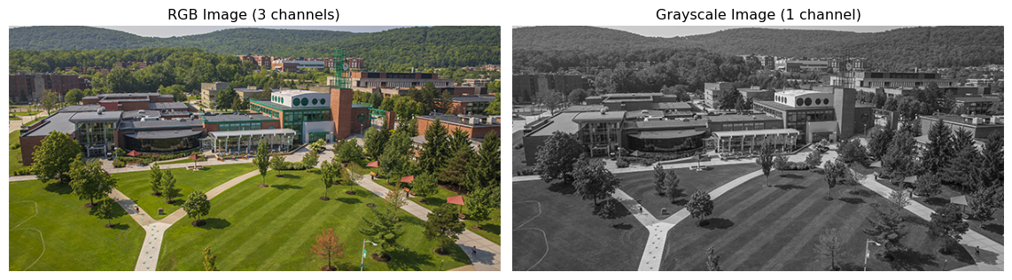
The grayscale version loses color information but preserves spatial structure. For many computer vision tasks, this simplified representation is sufficient.
When we feed images into neural networks, we need to be precise about dimensions. Different frameworks use different conventions. PyTorch expects images in (batch_size, channels, height, width) format, often abbreviated as NCHW:
Let’s convert our image to PyTorch format:
import torch

# Original numpy array is (H, W, C)
print(f"NumPy format (H, W, C): {img_array.shape}")

# Convert to PyTorch format (C, H, W) for a single image
img_tensor = torch.from_numpy(img_array).permute(2, 0, 1).float() / 255.0
print(f"PyTorch format (C, H, W): {img_tensor.shape}")

# Add batch dimension to get (N, C, H, W)
img_batch = img_tensor.unsqueeze(0)
print(f"Batch format (N, C, H, W): {img_batch.shape}")
NumPy format (H, W, C): (300, 600, 3)
PyTorch format (C, H, W): torch.Size([3, 300, 600])
Batch format (N, C, H, W): torch.Size([1, 3, 300, 600])We also normalized pixel values from [0, 255] to [0, 1] by dividing by 255. Why do this? This normalization helps neural networks train more stably.
Load your own image and explore its properties. Extract and visualize a small patch of pixels as numbers to see the underlying data structure. Modify some pixel values directly and observe how the image changes. Swap the red and blue channels to see the dramatic color shift this creates. Convert between NumPy and PyTorch formats to build fluency with both representations.
Understanding these representations at a hands-on level will make everything that follows more intuitive.
Now that we understand what images are as data structures, the next question becomes: how do we detect patterns in them? Human vision effortlessly recognizes edges, textures, and objects, but what computational operations allow machines to do the same? This question leads us to convolution, feature extraction, and ultimately to the deep learning revolution. In the next section, we’ll explore how computer vision evolved from hand-crafted feature detectors to learned representations that can match or exceed human performance. The key insight to carry forward is this: images are spatial data where relationships between neighboring pixels encode visual information.
We explored images as structured numerical data: a grayscale image is a 2D matrix of brightness values, while a color image adds two more matrices for the other color channels. Spatial relationships between pixels encode edges, textures, and objects, and unlike tabular data, the arrangement of values matters fundamentally. We saw how to load, inspect, and manipulate images in Python, converting between NumPy arrays and PyTorch tensors. This hands-on understanding prepares us to work with the deep learning models that process these image representations. Images are not just collections of numbers but spatially organized data where local patterns combine into global structure.